Flair NLP and flaiR for Social Science
Flair NLP is an open-source Natural Language Processing (NLP) library developed by Zalando Research. Known for its state-of-the-art solutions, it excels in contextual string embeddings, Named Entity Recognition (NER), and Part-of-Speech tagging (POS). Flair offers robust text analysis tools through multiple embedding approaches, including Flair contextual string embeddings, transformer-based embeddings from Hugging Face, and traditional models like GloVe and fasttext. Additionally, it provides pre-trained models for various languages and seamless integration with fine-tuned transformers hosted on Hugging Face.
flaiR bridges these powerful NLP features from Python to the R environment, making advanced text analysis accessible for social science researcher by combining Flair’s ease of use with R’s familiar interface for integration with popular R packages such as quanteda and more.
Sentence and Token
Sentence and Token are fundamental classes.
Sentence
A Sentence in Flair is an object that contains a sequence of Token objects, and it can be annotated with labels, such as named entities, part-of-speech tags, and more. It also can store embeddings for the sentence as a whole and different kinds of linguistic annotations.
Here’s a simple example of how you create a Sentence:
# Creating a Sentence object
library(flaiR)
string <- "What I see in UCD today, what I have seen of UCD in its impact on my own life and the life of Ireland."
Sentence <- flair_data()$Sentence
sentence <- Sentence(string)
Sentence[26] means that there are a total of 26 tokens
in the sentence.
print(sentence)
#> Sentence[26]: "What I see in UCD today, what I have seen of UCD in its impact on my own life and the life of Ireland."
Token
When you use Flair to handle text data,1 Sentence
and Token objects often play central roles in many use
cases. When you create a Sentence object, it automatically tokenizes the
text, removing the need to create the Token object manually.
Unlike R, which indexes from 1, Python indexes from 0. Therefore,
when using a for loop, I use seq_along(sentence) - 1. The
output should be something like:
# The Sentence object has automatically created and contains multiple Token objects
# We can iterate through the Sentence object to view each Token

for (i in seq_along(sentence)-1) {
  print(sentence[[i]])
}
#> Token[0]: "What"
#> Token[1]: "I"
#> Token[2]: "see"
#> Token[3]: "in"
#> Token[4]: "UCD"
#> Token[5]: "today"
#> Token[6]: ","
#> Token[7]: "what"
#> Token[8]: "I"
#> Token[9]: "have"
#> Token[10]: "seen"
#> Token[11]: "of"
#> Token[12]: "UCD"
#> Token[13]: "in"
#> Token[14]: "its"
#> Token[15]: "impact"
#> Token[16]: "on"
#> Token[17]: "my"
#> Token[18]: "own"
#> Token[19]: "life"
#> Token[20]: "and"
#> Token[21]: "the"
#> Token[22]: "life"
#> Token[23]: "of"
#> Token[24]: "Ireland"
#> Token[25]: "."
Or you can directly use $tokens method to print all
tokens.
print(sentence$tokens)
#> [[1]]
#> Token[0]: "What"
#>
#> [[2]]
#> Token[1]: "I"
#>
#> [[3]]
#> Token[2]: "see"
#>
#> [[4]]
#> Token[3]: "in"
#>
#> [[5]]
#> Token[4]: "UCD"
#>
#> [[6]]
#> Token[5]: "today"
#>
#> [[7]]
#> Token[6]: ","
#>
#> [[8]]
#> Token[7]: "what"
#>
#> [[9]]
#> Token[8]: "I"
#>
#> [[10]]
#> Token[9]: "have"
#>
#> [[11]]
#> Token[10]: "seen"
#>
#> [[12]]
#> Token[11]: "of"
#>
#> [[13]]
#> Token[12]: "UCD"
#>
#> [[14]]
#> Token[13]: "in"
#>
#> [[15]]
#> Token[14]: "its"
#>
#> [[16]]
#> Token[15]: "impact"
#>
#> [[17]]
#> Token[16]: "on"
#>
#> [[18]]
#> Token[17]: "my"
#>
#> [[19]]
#> Token[18]: "own"
#>
#> [[20]]
#> Token[19]: "life"
#>
#> [[21]]
#> Token[20]: "and"
#>
#> [[22]]
#> Token[21]: "the"
#>
#> [[23]]
#> Token[22]: "life"
#>
#> [[24]]
#> Token[23]: "of"
#>
#> [[25]]
#> Token[24]: "Ireland"
#>
#> [[26]]
#> Token[25]: "."
Retrieve the Token
To comprehend the string representation format of the Sentence
object, tagging at least one token is adequate. Python’s
get_token(n) method allows us to retrieve the Token object
for a particular token. Additionally, we can use
[] to index a specific token.
# method in Python
sentence$get_token(5)
#> Token[4]: "UCD"
# indexing in R
sentence[6]
#> Token[6]: ","
Each word (and punctuation) in the text is treated as an individual Token object. These Token objects store text information and other possible linguistic information (such as part-of-speech tags or named entity tags) and embedding (if you used a model to generate them).
While you do not need to create Token objects manually, understanding how to manage them is useful in situations where you might want to fine-tune the tokenization process. For example, you can control the exactness of tokenization by manually creating Token objects from a Sentence object.
This makes Flair very flexible when handling text data since the automatic tokenization feature can be used for rapid development, while also allowing users to fine-tune their tokenization.
Annotate POS tag and NER tag
The add_label(label_type, value) method can be employed
to assign a label to the token. In Universal POS tags, if
sentence[10] is ‘see’, ‘seen’ might be tagged as
VERB, indicating it is a past participle form of a
verb.
sentence[10]$add_label('manual-pos', 'VERB')
print(sentence[10])
#> Token[10]: "seen" → VERB (1.0000)
We can also add a NER (Named Entity Recognition) tag to
sentence[4], “UCD”, identifying it as a university in
Dublin.
sentence[4]$add_label('ner', 'ORG')
print(sentence[4])
#> Token[4]: "UCD" → ORG (1.0000)
If we print the sentence object, Sentence[50] provides
information for 50 tokens → [‘in’/ORG, ‘seen’/VERB], thus displaying two
tagging pieces of information.
print(sentence)
#> Sentence[26]: "What I see in UCD today, what I have seen of UCD in its impact on my own life and the life of Ireland." → ["UCD"/ORG, "seen"/VERB]
Corpus
The Corpus object in Flair is a fundamental data structure that represents a dataset containing text samples, usually comprising of a training set, a development set (or validation set), and a test set. It’s designed to work smoothly with Flair’s models for tasks like named entity recognition, text classification, and more.
Attributes:
-
train: A list of sentences (ListSentence) that form the training dataset. -
dev(or development): A list of sentences (ListSentence) that form the development (or validation) dataset. -
test: A list of sentences (ListSentence) that form the test dataset.
Important Methods:
-
downsample: This method allows you to downsample (reduce) the number of sentences in the train, dev, and test splits. -
obtain_statistics: This method gives a quick overview of the statistics of the corpus, including the number of sentences and the distribution of labels. -
make_vocab_dictionary: Used to create a vocabulary dictionary from the corpus.
library(flaiR)
Corpus <- flair_data()$Corpus
Sentence <- flair_data()$Sentence
# Create some example sentences
train <- list(Sentence('This is a training example.'))
dev <-  list(Sentence('This is a validation example.'))
test <- list(Sentence('This is a test example.'))

# Create a corpus using the custom data splits
corp <-  Corpus(train = train, dev = dev, test = test)
$obtain_statistics() method of the Corpus object in the
Flair library provides an overview of the dataset statistics. The method
returns a Python
dictionary with details about the training, validation
(development), and test datasets that make up the corpus. In R, you can
use the jsonlite package to format JSON.
library(jsonlite)
data <- fromJSON(corp$obtain_statistics())
formatted_str <- toJSON(data, pretty=TRUE)
print(formatted_str)
#> {
#>   "TRAIN": {
#>     "dataset": ["TRAIN"],
#>     "total_number_of_documents": [1],
#>     "number_of_documents_per_class": {},
#>     "number_of_tokens_per_tag": {},
#>     "number_of_tokens": {
#>       "total": [6],
#>       "min": [6],
#>       "max": [6],
#>       "avg": [6]
#>     }
#>   },
#>   "TEST": {
#>     "dataset": ["TEST"],
#>     "total_number_of_documents": [1],
#>     "number_of_documents_per_class": {},
#>     "number_of_tokens_per_tag": {},
#>     "number_of_tokens": {
#>       "total": [6],
#>       "min": [6],
#>       "max": [6],
#>       "avg": [6]
#>     }
#>   },
#>   "DEV": {
#>     "dataset": ["DEV"],
#>     "total_number_of_documents": [1],
#>     "number_of_documents_per_class": {},
#>     "number_of_tokens_per_tag": {},
#>     "number_of_tokens": {
#>       "total": [6],
#>       "min": [6],
#>       "max": [6],
#>       "avg": [6]
#>     }
#>   }
#> }
In R
Below, we use data from the article The Temporal Focus of Campaign Communication by Stefan Muller, published in the Journal of Politics in 2020, as an example.
First, we vectorize the cc_muller$text using the
Sentence function to transform it into a list object. Then, we reformat
cc_muller$class_pro_retro as a factor. It’s essential to
note that R handles numerical values differently than Python. In R,
numerical values are represented with a floating point, so it’s
advisable to convert them into factors or strings. Lastly, we employ the
map function from the purrr package to assign labels to each sentence
corpus using the $add_label method.
library(purrr)
#>
#> Attaching package: 'purrr'
#> The following object is masked from 'package:jsonlite':
#>
#>     flatten
data(cc_muller)
# The `Sentence` object tokenizes text
text <- lapply( cc_muller$text, Sentence)
# split sentence object to train and test.
labels <- as.factor(cc_muller$class_pro_retro)
# `$add_label` method assigns the corresponding coded type to each Sentence corpus.
text <- map2(text, labels, ~ .x$add_label("classification", .y), .progress = TRUE)
To perform a train-test split using base R, we can follow these steps:
set.seed(2046)
sample <- sample(c(TRUE, FALSE), length(text), replace=TRUE, prob=c(0.8, 0.2))
train  <- text[sample]
test   <- text[!sample]
sprintf("Corpus object sizes - Train: %d |  Test: %d", length(train), length(test))
#> [1] "Corpus object sizes - Train: 4710 |  Test: 1148"
If you don’t provide a dev set, flaiR will not force you to carve out a portion of your test set to serve as a dev set. However, in some cases when only the train and test sets are provided without a dev set, flaiR might automatically take a fraction of the train set (e.g., 10%) to use as a dev set (#2259). This is to offer a mechanism for model selection and to prevent the model from overfitting on the train set.
In the “Corpus” function, there is a random selection of the
"dev" dataset. To ensure reproducibility, we need to set
the seed in the flaiR framework. We can accomplish this by calling the
top-level module “flair” from flaiR and using
$set_seed(1964L) to set the seed.
flair <- import_flair()
flair$set_seed(1964L)
corp <- Corpus(train=train,
                 # dev=test,
                 test=test)
#> 2025-10-29 01:21:51,089 No dev split found. Using 10% (i.e. 471 samples) of the train split as dev data
sprintf("Corpus object sizes - Train: %d | Test: %d | Dev: %d",
        length(corp$train),
        length(corp$test),
        length(corp$dev))
#> [1] "Corpus object sizes - Train: 4239 | Test: 1148 | Dev: 471"
In the later sections, there will be more similar processing using
the Corpus. Following that, we will focus on advanced NLP
applications.
Sequence Taggings
Tag Entities in Text
Let’s run named entity recognition over the following example sentence: “I love Berlin and New York”. To do this, all you need to do is make a Sentence object for this text, load a pre-trained model and use it to predict tags for the object.
NER Models
| ID | Task | Language | Training Dataset | Accuracy | Contributor / Notes |
|---|---|---|---|---|---|
| ‘ner’ | NER (4-class) | English | Conll-03 | 93.03 (F1) | |
| ‘ner-fast’ | NER (4-class) | English | Conll-03 | 92.75 (F1) | (fast model) |
| ‘ner-large’ | NER (4-class) | English / Multilingual | Conll-03 | 94.09 (F1) | (large model) |
| ‘ner-pooled’ | NER (4-class) | English | Conll-03 | 93.24 (F1) | (memory inefficient) |
| ‘ner-ontonotes’ | NER (18-class) | English | Ontonotes | 89.06 (F1) | |
| ‘ner-ontonotes-fast’ | NER (18-class) | English | Ontonotes | 89.27 (F1) | (fast model) |
| ‘ner-ontonotes-large’ | NER (18-class) | English / Multilingual | Ontonotes | 90.93 (F1) | (large model) |
| ‘ar-ner’ | NER (4-class) | Arabic | AQMAR & ANERcorp (curated) | 86.66 (F1) | |
| ‘da-ner’ | NER (4-class) | Danish | Danish NER dataset | AmaliePauli | |
| ‘de-ner’ | NER (4-class) | German | Conll-03 | 87.94 (F1) | |
| ‘de-ner-large’ | NER (4-class) | German / Multilingual | Conll-03 | 92.31 (F1) | |
| ‘de-ner-germeval’ | NER (4-class) | German | Germeval | 84.90 (F1) | |
| ‘de-ner-legal’ | NER (legal text) | German | LER dataset | 96.35 (F1) | |
| ‘fr-ner’ | NER (4-class) | French | WikiNER (aij-wikiner-fr-wp3) | 95.57 (F1) | mhham |
| ‘es-ner-large’ | NER (4-class) | Spanish | CoNLL-03 | 90.54 (F1) | mhham |
| ‘nl-ner’ | NER (4-class) | Dutch | CoNLL 2002 | 92.58 (F1) | |
| ‘nl-ner-large’ | NER (4-class) | Dutch | Conll-03 | 95.25 (F1) | |
| ‘nl-ner-rnn’ | NER (4-class) | Dutch | CoNLL 2002 | 90.79 (F1) | |
| ‘ner-ukrainian’ | NER (4-class) | Ukrainian | NER-UK dataset | 86.05 (F1) | dchaplinsky |
Source: https://flairnlp.github.io/docs/tutorial-basics/tagging-entities
POS Models
| ID | Task | Language | Training Dataset | Accuracy | Contributor / Notes |
|---|---|---|---|---|---|
| ‘pos’ | POS-tagging | English | Ontonotes | 98.19 (Accuracy) | |
| ‘pos-fast’ | POS-tagging | English | Ontonotes | 98.1 (Accuracy) | (fast model) |
| ‘upos’ | POS-tagging (universal) | English | Ontonotes | 98.6 (Accuracy) | |
| ‘upos-fast’ | POS-tagging (universal) | English | Ontonotes | 98.47 (Accuracy) | (fast model) |
| ‘pos-multi’ | POS-tagging | Multilingual | UD Treebanks | 96.41 (average acc.) | (12 languages) |
| ‘pos-multi-fast’ | POS-tagging | Multilingual | UD Treebanks | 92.88 (average acc.) | (12 languages) |
| ‘ar-pos’ | POS-tagging | Arabic (+dialects) | combination of corpora | ||
| ‘de-pos’ | POS-tagging | German | UD German - HDT | 98.50 (Accuracy) | |
| ‘de-pos-tweets’ | POS-tagging | German | German Tweets | 93.06 (Accuracy) | stefan-it |
| ‘da-pos’ | POS-tagging | Danish | Danish Dependency Treebank | AmaliePauli | |
| ‘ml-pos’ | POS-tagging | Malayalam | 30000 Malayalam sentences | 83 | sabiqueqb |
| ‘ml-upos’ | POS-tagging | Malayalam | 30000 Malayalam sentences | 87 | sabiqueqb |
| ‘pt-pos-clinical’ | POS-tagging | Portuguese | PUCPR | 92.39 | LucasFerroHAILab for clinical texts |
| ‘pos-ukrainian’ | POS-tagging | Ukrainian | Ukrainian UD | 97.93 (F1) | dchaplinsky |
Source: https://flairnlp.github.io/docs/tutorial-basics/part-of-speech-tagging
# attach flaiR in R
library(flaiR)

# make a sentence

Sentence <- flair_data()$Sentence
sentence <- Sentence('I love Berlin and New York.')

# load the NER tagger
SequenceTagger <- flair_models()$SequenceTagger
tagger <- SequenceTagger$load('flair/ner-english')
#> 2025-10-29 01:21:51,628 SequenceTagger predicts: Dictionary with 20 tags: <unk>, O, S-ORG, S-MISC, B-PER, E-PER, S-LOC, B-ORG, E-ORG, I-PER, S-PER, B-MISC, I-MISC, E-MISC, I-ORG, B-LOC, E-LOC, I-LOC, <START>, <STOP>

# run NER over sentence
tagger$predict(sentence)
To print all annotations:
# print the sentence with all annotations
print(sentence)
#> Sentence[7]: "I love Berlin and New York." → ["Berlin"/LOC, "New York"/LOC]
Use a for loop to print out each POS tag. It’s important to note that
Python is indexed from 0. Therefore, in an R environment, we must use
seq_along(sentence$get_labels()) - 1.
Tag Part-of-Speech
We use flaiR/POS-english for POS tagging in the standard
models on Hugging Face.
# attach flaiR in R
library(flaiR)

# make a sentence
Sentence <- flair_data()$Sentence
sentence <- Sentence('I love Berlin and New York.')

# load the NER tagger
Classifier <- flair_nn()$Classifier
tagger <- Classifier$load('pos')
#> 2025-10-29 01:21:52,660 SequenceTagger predicts: Dictionary with 53 tags: <unk>, O, UH, ,, VBD, PRP, VB, PRP$, NN, RB, ., DT, JJ, VBP, VBG, IN, CD, NNS, NNP, WRB, VBZ, WDT, CC, TO, MD, VBN, WP, :, RP, EX, JJR, FW, XX, HYPH, POS, RBR, JJS, PDT, NNPS, RBS, AFX, WP$, -LRB-, -RRB-, ``, '', LS, $, SYM, ADD
Penn Treebank POS Tags Reference
| Tag | Description | Example |
|---|---|---|
| DT | Determiner | the, a, these |
| NN | Noun, singular | cat, tree |
| NNS | Noun, plural | cats, trees |
| NNP | Proper noun, singular | John, London |
| NNPS | Proper noun, plural | Americans |
| VB | Verb, base form | take |
| VBD | Verb, past tense | took |
| VBG | Verb, gerund/present participle | taking |
| VBN | Verb, past participle | taken |
| VBP | Verb, non-3rd person singular present | take |
| VBZ | Verb, 3rd person singular present | takes |
| JJ | Adjective | big |
| RB | Adverb | quickly |
| O | Other | - |
| , | Comma | , |
| . | Period | . |
| : | Colon | : |
| -LRB- | Left bracket | ( |
| -RRB- | Right bracket | ) |
| `` | Opening quotation | ” |
| ’’ | Closing quotation | ” |
| HYPH | Hyphen | - |
| CD | Cardinal number | 1, 2, 3 |
| IN | Preposition | in, on, at |
| PRP | Personal pronoun | I, you, he |
| PRP$ | Possessive pronoun | my, your |
| UH | Interjection | oh, wow |
| FW | Foreign word | café |
| SYM | Symbol | +, % |
# run NER over sentence
tagger$predict(sentence)
# print the sentence with all annotations
print(sentence)
#> Sentence[7]: "I love Berlin and New York." → ["I"/PRP, "love"/VBP, "Berlin"/NNP, "and"/CC, "New"/NNP, "York"/NNP, "."/.]
Use a for loop to print out each POS tag.
for (i in seq_along(sentence$get_labels())) {
      print(sentence$get_labels()[[i]])
  }
#> 'Token[0]: "I"'/'PRP' (1.0)
#> 'Token[1]: "love"'/'VBP' (1.0)
#> 'Token[2]: "Berlin"'/'NNP' (0.9999)
#> 'Token[3]: "and"'/'CC' (1.0)
#> 'Token[4]: "New"'/'NNP' (1.0)
#> 'Token[5]: "York"'/'NNP' (1.0)
#> 'Token[6]: "."'/'.' (1.0)
Detect Sentiment
Let’s run sentiment analysis over the same sentence to determine whether it is POSITIVE or NEGATIVE.
You can do this with essentially the same code as above. Instead of
loading the ‘ner’ model, you now load the 'sentiment'
model:
# attach flaiR in R
library(flaiR)

# make a sentence
Sentence <- flair_data()$Sentence
sentence <- Sentence('I love Berlin and New York.')

# load the Classifier tagger from flair.nn module
Classifier <- flair_nn()$Classifier
tagger <- Classifier$load('sentiment')

# run sentiment analysis over sentence
tagger$predict(sentence)
# print the sentence with all annotations
print(sentence)
#> Sentence[7]: "I love Berlin and New York." → POSITIVE (0.9982)
Dealing with Dataframe
Parts-of-Speech Tagging Across Full DataFrame
You can apply Part-of-Speech (POS) tagging across an entire DataFrame using Flair’s pre-trained models. Let’s walk through an example using the pos-fast model. You can apply Part-of-Speech (POS) tagging across an entire DataFrame using Flair’s pre-trained models. Let’s walk through an example using the pos-fast model. First, let’s load our required packages and sample data:
For POS tagging, we’ll use Flair’s pre-trained model. The pos-fast model offers a good balance between speed and accuracy. For more pre-trained models, check out Flair’s documentation at Flair POS Tagging Documentation. There are two ways to load the POS tagger:
- Load with tag dictionary display (default):
tagger_pos <- load_tagger_pos("pos-fast")
#> Loading POS tagger model: pos-fast
#> 2025-10-29 01:21:55,936 SequenceTagger predicts: Dictionary with 53 tags: <unk>, O, UH, ,, VBD, PRP, VB, PRP$, NN, RB, ., DT, JJ, VBP, VBG, IN, CD, NNS, NNP, WRB, VBZ, WDT, CC, TO, MD, VBN, WP, :, RP, EX, JJR, FW, XX, HYPH, POS, RBR, JJS, PDT, NNPS, RBS, AFX, WP$, -LRB-, -RRB-, ``, '', LS, $, SYM, ADD
#>
#> POS Tagger Dictionary:
#> ========================================
#> Total tags: 53
#> ----------------------------------------
#> Special:       <unk>, O, <START>, <STOP>
#> Nouns:         PRP, PRP$, NN, NNS, NNP, WP, EX, NNPS, WP$
#> Verbs:         VBD, VB, VBP, VBG, VBZ, MD, VBN
#> Adjectives:    JJ, JJR, POS, JJS
#> Adverbs:       RB, WRB, RBR, RBS
#> Determiners:   DT, WDT, PDT
#> Prepositions:  IN, TO
#> Conjunctions:  CC
#> Numbers:       CD
#> Punctuation:   <unk>, ,, ., :, HYPH, -LRB-, -RRB-, ``, '', $, NFP, <START>, <STOP>
#> Others:        UH, FW, XX, LS, $, SYM, ADD
#> ----------------------------------------
#> Common POS Tag Meanings:
#> NN*: Nouns (NNP: Proper, NNS: Plural)
#> VB*: Verbs (VBD: Past, VBG: Gerund)
#> JJ*: Adjectives (JJR: Comparative)
#> RB*: Adverbs
#> PRP: Pronouns, DT: Determiners
#> IN: Prepositions, CC: Conjunctions
#> ========================================
This will show you all available POS tags grouped by categories (nouns, verbs, adjectives, etc.).
- Load without tag display for a cleaner output:
pos_tagger <- load_tagger_pos("pos-fast", show_tags = FALSE)
#> Loading POS tagger model: pos-fast
#> 2025-10-29 01:21:56,318 SequenceTagger predicts: Dictionary with 53 tags: <unk>, O, UH, ,, VBD, PRP, VB, PRP$, NN, RB, ., DT, JJ, VBP, VBG, IN, CD, NNS, NNP, WRB, VBZ, WDT, CC, TO, MD, VBN, WP, :, RP, EX, JJR, FW, XX, HYPH, POS, RBR, JJS, PDT, NNPS, RBS, AFX, WP$, -LRB-, -RRB-, ``, '', LS, $, SYM, ADD
Now we can process our texts:
results <- get_pos(texts = uk_immigration$text,
                   doc_ids = uk_immigration$speaker,
                   show.text_id = TRUE,
                   tagger = pos_tagger)

head(results, n = 10)
#>               doc_id token_id
#>               <char>    <num>
#>  1: Philip Hollobone        0
#>  2: Philip Hollobone        1
#>  3: Philip Hollobone        2
#>  4: Philip Hollobone        3
#>  5: Philip Hollobone        4
#>  6: Philip Hollobone        5
#>  7: Philip Hollobone        6
#>  8: Philip Hollobone        7
#>  9: Philip Hollobone        8
#> 10: Philip Hollobone        9
#>                                                                                                                                                                                                                                                                                                                                                                                                                                                                                                                                                                                                                                                                                                                                                                                                                                                                                                                                                                                                                                                                                                                                                                                                                                                                                                                                                                                                                                                                                                                                                                                                                                                                                                                                                                                                                                                                                                                                                                                                                                                                                                                   text_id
#>                                                                                                                                                                                                                                                                                                                                                                                                                                                                                                                                                                                                                                                                                                                                                                                                                                                                                                                                                                                                                                                                                                                                                                                                                                                                                                                                                                                                                                                                                                                                                                                                                                                                                                                                                                                                                                                                                                                                                                                                                                                                                                                    <char>
#>  1: I thank Mr. Speaker for giving me permission to hold this debate today. I welcome the Minister-I very much appreciate the contact from his office prior to today-and the Conservative and Liberal Democrat Front Benchers to the debate. I also welcome my hon. Friends on the Back Benches. Immigration is the most important issue for my constituents. I get more complaints, comments and suggestions about immigration than about anything else. In the Kettering constituency, the number of immigrants is actually very low. There is a well-settled Sikh community in the middle of Kettering town itself, which has been in Kettering for some 40 or 50 years and is very much part of the local community and of the fabric of local life. There are other very small migrant groups in my constituency, but it is predominantly made up of indigenous British people. However, there is huge concern among my constituents about the level of immigration into our country. I believe that I am right in saying that, in recent years, net immigration into the United Kingdom is the largest wave of immigration that our country has ever known and, proportionately, is probably the biggest wave of immigration since the Norman conquest. My contention is that our country simply cannot cope with immigration on that scale-to coin a phrase, we simply cannot go on like this. It is about time that mainstream politicians started airing the views of their constituents, because for too long people have muttered under their breath that they are concerned about immigration. They have been frightened to speak out about it because they are frightened of being accused of being racist. My contention is that immigration is not a racist issue; it is a question of numbers. I personally could not care tuppence about the ethnicity of the immigrants concerned, the colour of their skin or the language that they speak. What I am concerned about is the very large numbers of new arrivals to our country. My contention is that the United Kingdom simply cannot cope with them.
#>  2: I thank Mr. Speaker for giving me permission to hold this debate today. I welcome the Minister-I very much appreciate the contact from his office prior to today-and the Conservative and Liberal Democrat Front Benchers to the debate. I also welcome my hon. Friends on the Back Benches. Immigration is the most important issue for my constituents. I get more complaints, comments and suggestions about immigration than about anything else. In the Kettering constituency, the number of immigrants is actually very low. There is a well-settled Sikh community in the middle of Kettering town itself, which has been in Kettering for some 40 or 50 years and is very much part of the local community and of the fabric of local life. There are other very small migrant groups in my constituency, but it is predominantly made up of indigenous British people. However, there is huge concern among my constituents about the level of immigration into our country. I believe that I am right in saying that, in recent years, net immigration into the United Kingdom is the largest wave of immigration that our country has ever known and, proportionately, is probably the biggest wave of immigration since the Norman conquest. My contention is that our country simply cannot cope with immigration on that scale-to coin a phrase, we simply cannot go on like this. It is about time that mainstream politicians started airing the views of their constituents, because for too long people have muttered under their breath that they are concerned about immigration. They have been frightened to speak out about it because they are frightened of being accused of being racist. My contention is that immigration is not a racist issue; it is a question of numbers. I personally could not care tuppence about the ethnicity of the immigrants concerned, the colour of their skin or the language that they speak. What I am concerned about is the very large numbers of new arrivals to our country. My contention is that the United Kingdom simply cannot cope with them.
#>  3: I thank Mr. Speaker for giving me permission to hold this debate today. I welcome the Minister-I very much appreciate the contact from his office prior to today-and the Conservative and Liberal Democrat Front Benchers to the debate. I also welcome my hon. Friends on the Back Benches. Immigration is the most important issue for my constituents. I get more complaints, comments and suggestions about immigration than about anything else. In the Kettering constituency, the number of immigrants is actually very low. There is a well-settled Sikh community in the middle of Kettering town itself, which has been in Kettering for some 40 or 50 years and is very much part of the local community and of the fabric of local life. There are other very small migrant groups in my constituency, but it is predominantly made up of indigenous British people. However, there is huge concern among my constituents about the level of immigration into our country. I believe that I am right in saying that, in recent years, net immigration into the United Kingdom is the largest wave of immigration that our country has ever known and, proportionately, is probably the biggest wave of immigration since the Norman conquest. My contention is that our country simply cannot cope with immigration on that scale-to coin a phrase, we simply cannot go on like this. It is about time that mainstream politicians started airing the views of their constituents, because for too long people have muttered under their breath that they are concerned about immigration. They have been frightened to speak out about it because they are frightened of being accused of being racist. My contention is that immigration is not a racist issue; it is a question of numbers. I personally could not care tuppence about the ethnicity of the immigrants concerned, the colour of their skin or the language that they speak. What I am concerned about is the very large numbers of new arrivals to our country. My contention is that the United Kingdom simply cannot cope with them.
#>  4: I thank Mr. Speaker for giving me permission to hold this debate today. I welcome the Minister-I very much appreciate the contact from his office prior to today-and the Conservative and Liberal Democrat Front Benchers to the debate. I also welcome my hon. Friends on the Back Benches. Immigration is the most important issue for my constituents. I get more complaints, comments and suggestions about immigration than about anything else. In the Kettering constituency, the number of immigrants is actually very low. There is a well-settled Sikh community in the middle of Kettering town itself, which has been in Kettering for some 40 or 50 years and is very much part of the local community and of the fabric of local life. There are other very small migrant groups in my constituency, but it is predominantly made up of indigenous British people. However, there is huge concern among my constituents about the level of immigration into our country. I believe that I am right in saying that, in recent years, net immigration into the United Kingdom is the largest wave of immigration that our country has ever known and, proportionately, is probably the biggest wave of immigration since the Norman conquest. My contention is that our country simply cannot cope with immigration on that scale-to coin a phrase, we simply cannot go on like this. It is about time that mainstream politicians started airing the views of their constituents, because for too long people have muttered under their breath that they are concerned about immigration. They have been frightened to speak out about it because they are frightened of being accused of being racist. My contention is that immigration is not a racist issue; it is a question of numbers. I personally could not care tuppence about the ethnicity of the immigrants concerned, the colour of their skin or the language that they speak. What I am concerned about is the very large numbers of new arrivals to our country. My contention is that the United Kingdom simply cannot cope with them.
#>  5: I thank Mr. Speaker for giving me permission to hold this debate today. I welcome the Minister-I very much appreciate the contact from his office prior to today-and the Conservative and Liberal Democrat Front Benchers to the debate. I also welcome my hon. Friends on the Back Benches. Immigration is the most important issue for my constituents. I get more complaints, comments and suggestions about immigration than about anything else. In the Kettering constituency, the number of immigrants is actually very low. There is a well-settled Sikh community in the middle of Kettering town itself, which has been in Kettering for some 40 or 50 years and is very much part of the local community and of the fabric of local life. There are other very small migrant groups in my constituency, but it is predominantly made up of indigenous British people. However, there is huge concern among my constituents about the level of immigration into our country. I believe that I am right in saying that, in recent years, net immigration into the United Kingdom is the largest wave of immigration that our country has ever known and, proportionately, is probably the biggest wave of immigration since the Norman conquest. My contention is that our country simply cannot cope with immigration on that scale-to coin a phrase, we simply cannot go on like this. It is about time that mainstream politicians started airing the views of their constituents, because for too long people have muttered under their breath that they are concerned about immigration. They have been frightened to speak out about it because they are frightened of being accused of being racist. My contention is that immigration is not a racist issue; it is a question of numbers. I personally could not care tuppence about the ethnicity of the immigrants concerned, the colour of their skin or the language that they speak. What I am concerned about is the very large numbers of new arrivals to our country. My contention is that the United Kingdom simply cannot cope with them.
#>  6: I thank Mr. Speaker for giving me permission to hold this debate today. I welcome the Minister-I very much appreciate the contact from his office prior to today-and the Conservative and Liberal Democrat Front Benchers to the debate. I also welcome my hon. Friends on the Back Benches. Immigration is the most important issue for my constituents. I get more complaints, comments and suggestions about immigration than about anything else. In the Kettering constituency, the number of immigrants is actually very low. There is a well-settled Sikh community in the middle of Kettering town itself, which has been in Kettering for some 40 or 50 years and is very much part of the local community and of the fabric of local life. There are other very small migrant groups in my constituency, but it is predominantly made up of indigenous British people. However, there is huge concern among my constituents about the level of immigration into our country. I believe that I am right in saying that, in recent years, net immigration into the United Kingdom is the largest wave of immigration that our country has ever known and, proportionately, is probably the biggest wave of immigration since the Norman conquest. My contention is that our country simply cannot cope with immigration on that scale-to coin a phrase, we simply cannot go on like this. It is about time that mainstream politicians started airing the views of their constituents, because for too long people have muttered under their breath that they are concerned about immigration. They have been frightened to speak out about it because they are frightened of being accused of being racist. My contention is that immigration is not a racist issue; it is a question of numbers. I personally could not care tuppence about the ethnicity of the immigrants concerned, the colour of their skin or the language that they speak. What I am concerned about is the very large numbers of new arrivals to our country. My contention is that the United Kingdom simply cannot cope with them.
#>  7: I thank Mr. Speaker for giving me permission to hold this debate today. I welcome the Minister-I very much appreciate the contact from his office prior to today-and the Conservative and Liberal Democrat Front Benchers to the debate. I also welcome my hon. Friends on the Back Benches. Immigration is the most important issue for my constituents. I get more complaints, comments and suggestions about immigration than about anything else. In the Kettering constituency, the number of immigrants is actually very low. There is a well-settled Sikh community in the middle of Kettering town itself, which has been in Kettering for some 40 or 50 years and is very much part of the local community and of the fabric of local life. There are other very small migrant groups in my constituency, but it is predominantly made up of indigenous British people. However, there is huge concern among my constituents about the level of immigration into our country. I believe that I am right in saying that, in recent years, net immigration into the United Kingdom is the largest wave of immigration that our country has ever known and, proportionately, is probably the biggest wave of immigration since the Norman conquest. My contention is that our country simply cannot cope with immigration on that scale-to coin a phrase, we simply cannot go on like this. It is about time that mainstream politicians started airing the views of their constituents, because for too long people have muttered under their breath that they are concerned about immigration. They have been frightened to speak out about it because they are frightened of being accused of being racist. My contention is that immigration is not a racist issue; it is a question of numbers. I personally could not care tuppence about the ethnicity of the immigrants concerned, the colour of their skin or the language that they speak. What I am concerned about is the very large numbers of new arrivals to our country. My contention is that the United Kingdom simply cannot cope with them.
#>  8: I thank Mr. Speaker for giving me permission to hold this debate today. I welcome the Minister-I very much appreciate the contact from his office prior to today-and the Conservative and Liberal Democrat Front Benchers to the debate. I also welcome my hon. Friends on the Back Benches. Immigration is the most important issue for my constituents. I get more complaints, comments and suggestions about immigration than about anything else. In the Kettering constituency, the number of immigrants is actually very low. There is a well-settled Sikh community in the middle of Kettering town itself, which has been in Kettering for some 40 or 50 years and is very much part of the local community and of the fabric of local life. There are other very small migrant groups in my constituency, but it is predominantly made up of indigenous British people. However, there is huge concern among my constituents about the level of immigration into our country. I believe that I am right in saying that, in recent years, net immigration into the United Kingdom is the largest wave of immigration that our country has ever known and, proportionately, is probably the biggest wave of immigration since the Norman conquest. My contention is that our country simply cannot cope with immigration on that scale-to coin a phrase, we simply cannot go on like this. It is about time that mainstream politicians started airing the views of their constituents, because for too long people have muttered under their breath that they are concerned about immigration. They have been frightened to speak out about it because they are frightened of being accused of being racist. My contention is that immigration is not a racist issue; it is a question of numbers. I personally could not care tuppence about the ethnicity of the immigrants concerned, the colour of their skin or the language that they speak. What I am concerned about is the very large numbers of new arrivals to our country. My contention is that the United Kingdom simply cannot cope with them.
#>  9: I thank Mr. Speaker for giving me permission to hold this debate today. I welcome the Minister-I very much appreciate the contact from his office prior to today-and the Conservative and Liberal Democrat Front Benchers to the debate. I also welcome my hon. Friends on the Back Benches. Immigration is the most important issue for my constituents. I get more complaints, comments and suggestions about immigration than about anything else. In the Kettering constituency, the number of immigrants is actually very low. There is a well-settled Sikh community in the middle of Kettering town itself, which has been in Kettering for some 40 or 50 years and is very much part of the local community and of the fabric of local life. There are other very small migrant groups in my constituency, but it is predominantly made up of indigenous British people. However, there is huge concern among my constituents about the level of immigration into our country. I believe that I am right in saying that, in recent years, net immigration into the United Kingdom is the largest wave of immigration that our country has ever known and, proportionately, is probably the biggest wave of immigration since the Norman conquest. My contention is that our country simply cannot cope with immigration on that scale-to coin a phrase, we simply cannot go on like this. It is about time that mainstream politicians started airing the views of their constituents, because for too long people have muttered under their breath that they are concerned about immigration. They have been frightened to speak out about it because they are frightened of being accused of being racist. My contention is that immigration is not a racist issue; it is a question of numbers. I personally could not care tuppence about the ethnicity of the immigrants concerned, the colour of their skin or the language that they speak. What I am concerned about is the very large numbers of new arrivals to our country. My contention is that the United Kingdom simply cannot cope with them.
#> 10: I thank Mr. Speaker for giving me permission to hold this debate today. I welcome the Minister-I very much appreciate the contact from his office prior to today-and the Conservative and Liberal Democrat Front Benchers to the debate. I also welcome my hon. Friends on the Back Benches. Immigration is the most important issue for my constituents. I get more complaints, comments and suggestions about immigration than about anything else. In the Kettering constituency, the number of immigrants is actually very low. There is a well-settled Sikh community in the middle of Kettering town itself, which has been in Kettering for some 40 or 50 years and is very much part of the local community and of the fabric of local life. There are other very small migrant groups in my constituency, but it is predominantly made up of indigenous British people. However, there is huge concern among my constituents about the level of immigration into our country. I believe that I am right in saying that, in recent years, net immigration into the United Kingdom is the largest wave of immigration that our country has ever known and, proportionately, is probably the biggest wave of immigration since the Norman conquest. My contention is that our country simply cannot cope with immigration on that scale-to coin a phrase, we simply cannot go on like this. It is about time that mainstream politicians started airing the views of their constituents, because for too long people have muttered under their breath that they are concerned about immigration. They have been frightened to speak out about it because they are frightened of being accused of being racist. My contention is that immigration is not a racist issue; it is a question of numbers. I personally could not care tuppence about the ethnicity of the immigrants concerned, the colour of their skin or the language that they speak. What I am concerned about is the very large numbers of new arrivals to our country. My contention is that the United Kingdom simply cannot cope with them.
#>          token    tag  score
#>         <char> <char>  <num>
#>  1:          I    PRP 1.0000
#>  2:      thank    VBP 0.9992
#>  3:        Mr.    NNP 1.0000
#>  4:    Speaker    NNP 1.0000
#>  5:        for     IN 1.0000
#>  6:     giving    VBG 1.0000
#>  7:         me    PRP 1.0000
#>  8: permission     NN 0.9999
#>  9:         to     TO 0.9999
#> 10:       hold     VB 1.0000
Tagging Entities Across Full DataFrame
This section focuses on performing Named Entity Recognition (NER) on data stored in a dataframe format. My goal is to identify and tag named entities within text that is organized in a structured dataframe.
I load the flaiR package and use the built-in uk_immigration dataset. For demonstration purposes, I’m only taking the first two rows. This dataset contains discussions about immigration in the UK.
Load the pre-trained model ner. For more pre-trained
models, see https://flairnlp.github.io/docs/tutorial-basics/tagging-entities.
Next, I load the latest model hosted and maintained on Hugging Face by the Flair NLP team. For more Flair NER models, you can visit the official Flair NLP page on Hugging Face (https://huggingface.co/flair).
# Load model without displaying tags
# tagger <- load_tagger_ner("flair/ner-english-large", show_tags = FALSE)

library(flaiR)
tagger_ner <- load_tagger_ner("flair/ner-english-ontonotes")
#> 2025-10-29 01:22:01,578 SequenceTagger predicts: Dictionary with 75 tags: O, S-PERSON, B-PERSON, E-PERSON, I-PERSON, S-GPE, B-GPE, E-GPE, I-GPE, S-ORG, B-ORG, E-ORG, I-ORG, S-DATE, B-DATE, E-DATE, I-DATE, S-CARDINAL, B-CARDINAL, E-CARDINAL, I-CARDINAL, S-NORP, B-NORP, E-NORP, I-NORP, S-MONEY, B-MONEY, E-MONEY, I-MONEY, S-PERCENT, B-PERCENT, E-PERCENT, I-PERCENT, S-ORDINAL, B-ORDINAL, E-ORDINAL, I-ORDINAL, S-LOC, B-LOC, E-LOC, I-LOC, S-TIME, B-TIME, E-TIME, I-TIME, S-WORK_OF_ART, B-WORK_OF_ART, E-WORK_OF_ART, I-WORK_OF_ART, S-FAC
#>
#> NER Tagger Dictionary:
#> ========================================
#> Total tags: 75
#> Model: flair/ner-english-ontonotes
#> ----------------------------------------
#> Special        : O, <START>, <STOP>
#> Person         : S-PERSON, B-PERSON, E-PERSON, I-PERSON
#> Organization   : S-ORG, B-ORG, E-ORG, I-ORG
#> Location       : S-GPE, B-GPE, E-GPE, I-GPE, S-LOC, B-LOC, E-LOC, I-LOC
#> Time           : S-DATE, B-DATE, E-DATE, I-DATE, S-TIME, B-TIME, E-TIME, I-TIME
#> Numbers        : S-CARDINAL, B-CARDINAL, E-CARDINAL, I-CARDINAL, S-MONEY, B-MONEY, E-MONEY, I-MONEY, S-PERCENT, B-PERCENT, E-PERCENT, I-PERCENT, S-ORDINAL, B-ORDINAL, E-ORDINAL, I-ORDINAL
#> Groups         : S-NORP, B-NORP, E-NORP, I-NORP
#> Facilities     : S-FAC, B-FAC, E-FAC, I-FAC
#> Products       : S-PRODUCT, B-PRODUCT, E-PRODUCT, I-PRODUCT
#> Events         : S-EVENT, B-EVENT, E-EVENT, I-EVENT
#> Art            : S-WORK_OF_ART, B-WORK_OF_ART, E-WORK_OF_ART, I-WORK_OF_ART
#> Languages      : S-LANGUAGE, B-LANGUAGE, E-LANGUAGE, I-LANGUAGE
#> Laws           : S-LAW, B-LAW, E-LAW, I-LAW
#> ----------------------------------------
#> Tag scheme: BIOES
#> B-: Beginning of multi-token entity
#> I-: Inside of multi-token entity
#> O: Outside (not part of any entity)
#> E-: End of multi-token entity
#> S-: Single token entity
#> ========================================
I load a pre-trained NER model. Since I’m using a Mac M1/M2, I set the model to run on the MPS device for faster processing. If I want to use other pre-trained models, I can check the Flair documentation website for available options.
Now I’m ready to process the text:
results <- get_entities(texts = uk_immigration$text,
                        doc_ids = uk_immigration$speaker,
                        tagger = tagger_ner,
                        batch_size = 2,
                        verbose = FALSE)
#> CPU is used.
head(results, n = 10)
#>               doc_id                          entity    tag     score
#>               <char>                          <char> <char>     <num>
#>  1: Philip Hollobone                           today   DATE 0.9843613
#>  2: Philip Hollobone                    Conservative   NORP 0.9976857
#>  3: Philip Hollobone Liberal Democrat Front Benchers    ORG 0.7668477
#>  4: Philip Hollobone                       Kettering    GPE 0.9885774
#>  5: Philip Hollobone                            Sikh   NORP 0.9939976
#>  6: Philip Hollobone                       Kettering    GPE 0.9955219
#>  7: Philip Hollobone                       Kettering    GPE 0.9948049
#>  8: Philip Hollobone             some 40 or 50 years   DATE 0.8059650
#>  9: Philip Hollobone                         British   NORP 0.9986913
#> 10: Philip Hollobone                    recent years   DATE 0.8596769
Highlight Entities with Colors
This tutorial demonstrates how to use the flaiR package to identify and highlight named entities (such as names, locations, organizations) in text.
Step 1 Create Text with Named Entities
First, we load the flaiR package and work with a sample text:
library(flaiR)
data("uk_immigration")
uk_immigration <- uk_immigration[30,]
tagger_ner <- load_tagger_ner("flair/ner-english-fast")
#> 2025-10-29 01:22:09,213 SequenceTagger predicts: Dictionary with 20 tags: <unk>, O, S-ORG, S-MISC, B-PER, E-PER, S-LOC, B-ORG, E-ORG, I-PER, S-PER, B-MISC, I-MISC, E-MISC, I-ORG, B-LOC, E-LOC, I-LOC, <START>, <STOP>
#>
#> NER Tagger Dictionary:
#> ========================================
#> Total tags: 20
#> Model: flair/ner-english-fast
#> ----------------------------------------
#> Special        : <unk>, O, <START>, <STOP>
#> Organization   : S-ORG, B-ORG, E-ORG, I-ORG
#> Location       : S-LOC, B-LOC, E-LOC, I-LOC
#> Misc           : S-MISC, B-MISC, I-MISC, E-MISC
#> ----------------------------------------
#> Tag scheme: BIOES
#> B-: Beginning of multi-token entity
#> I-: Inside of multi-token entity
#> O: Outside (not part of any entity)
#> E-: End of multi-token entity
#> S-: Single token entity
#> ========================================

result <- get_entities(uk_immigration$text,
                       tagger = tagger_ner,
                       show.text_id = FALSE
                       )
#> CPU is used.
#> Warning in check_texts_and_ids(texts, doc_ids): doc_ids is NULL.
#> Auto-assigning doc_ids.
Step 2 Highlight the Named Entities
Use the highlight_text function to color-code the
identified entities:
highlighted_text <- highlight_text(text = uk_immigration$text,
                                   entities_mapping = map_entities(result))
highlighted_textExplanation:
-
load_tagger_ner("ner")loads the pre-trained NER model -
get_entities()identifies named entities in the text -
map_entities()maps the identified entities to colors -
highlight_text()marks the original text using these colors
Each type of entity (such as person names, locations, organization names) will be displayed in a different color, making the named entities in the text immediately visible.
The Overview of Embedding
All word embedding classes inherit from the
TokenEmbeddings class and call the embed()
method to embed the text. In most cases when using Flair, various and
complex embedding processes are hidden behind the interface. Users
simply need to instantiate the necessary embedding class and call
embed() to embed text.
Here are the types of embeddings currently supported in FlairNLP:
| Class | Type | Paper |
|---|---|---|
BytePairEmbeddings |
Subword-level word embeddings | Heinzerling and Strube (2018) |
CharacterEmbeddings |
Task-trained character-level embeddings of words | Lample et al. (2016) |
ELMoEmbeddings |
Contextualized word-level embeddings | Peters et al. (2018) |
FastTextEmbeddings |
Word embeddings with subword features | Bojanowski et al. (2017) |
FlairEmbeddings |
Contextualized character-level embeddings | Akbik et al. (2018) |
OneHotEmbeddings |
Standard one-hot embeddings of text or tags | - |
PooledFlairEmbeddings |
Pooled variant of FlairEmbeddings
|
Akbik et al. (2019) |
TransformerWordEmbeddings) |
Embeddings from pretrained transformers (BERT, XLM, GPT, RoBERTa, XLNet, DistilBERT etc.) | Devlin et al. (2018) Radford et al. (2018) Liu et al. (2019) Dai et al. (2019) Yang et al. (2019) Lample and Conneau (2019) |
WordEmbeddings |
Classic word embeddings |
Byte Pair Embeddings
Please note that ihis document for R is a conversion of the Flair NLP document implemented in Python.
BytePairEmbeddings are word embeddings that operate at
the subword level. They can embed any word by breaking it down into
subwords and looking up their corresponding embeddings. This technique
was introduced by Heinzerling and Strube
(2018) , who demonstrated that BytePairEmbeddings achieve comparable
accuracy to traditional word embeddings while requiring only a fraction
of the model size. This makes them an excellent choice for training
compact models.
To initialize BytePairEmbeddings, you need to specify:
- A language code (275 languages supported)
- Number of syllables
- Number of dimensions (options: 50, 100, 200, or 300)
library(flaiR)

# Initialize embedding
BytePairEmbeddings <- flair_embeddings()$BytePairEmbeddings

# Create BytePairEmbeddings with specified parameters
embedding <- BytePairEmbeddings(
    language = "en",        # Language code (e.g., "en" for English)
    dim = 50L,              # Embedding dimensions: options are 50L, 100L, 200L, or 300L
    syllables = 100000L     # Subword vocabulary size

)

# Create a sample sentence
Sentence <- flair_data()$Sentence
sentence = Sentence('The grass is green .')

# Embed words in the sentence
embedding$embed(sentence)
#> [[1]]
#> Sentence[5]: "The grass is green ."

# Print embeddings
for (i in 1:length(sentence$tokens)) {
    token <- sentence$tokens[[i]]
    cat("\nWord:", token$text, "\n")

    # Convert embedding to R vector and print
    # Python index starts from 0, so use i-1
    embedding_vector <- sentence[i-1]$embedding$numpy()
    cat("Embedding shape:", length(embedding_vector), "\n")
    cat("First 5 values:", head(embedding_vector, 5), "\n")
    cat("-------------------\n")
}
#>
#> Word: The
#> Embedding shape: 100
#> First 5 values: -0.585645 0.55233 -0.335385 -0.117119 -0.3433
#> -------------------
#>
#> Word: grass
#> Embedding shape: 100
#> First 5 values: 0.370427 -0.717806 -0.489089 0.384228 0.68443
#> -------------------
#>
#> Word: is
#> Embedding shape: 100
#> First 5 values: -0.186592 0.52804 -1.011618 0.416936 -0.166446
#> -------------------
#>
#> Word: green
#> Embedding shape: 100
#> First 5 values: -0.075467 -0.874228 0.20425 1.061623 -0.246111
#> -------------------
#>
#> Word: .
#> Embedding shape: 100
#> First 5 values: -0.214652 0.212236 -0.607079 0.512853 -0.325556
#> -------------------
More information can be found on the byte pair embeddings web page.
BytePairEmbeddings also have a multilingual model capable
of embedding any word in any language. You can instantiate it with:
embedding <- BytePairEmbeddings('multi')You can also load custom BytePairEmbeddings by
specifying a path to model_file_path and embedding_file_path arguments.
They correspond respectively to a SentencePiece model file
and to an embedding file (Word2Vec plain text or GenSim binary).
Flair Embeddings
The following example manual is translated into R from Flair NLP by Zalando Research. In Flair, the use of embedding is very quite straightforward. Here’s an example code snippet of how to use Flair’s contextual string embeddings:
library(flaiR)
FlairEmbeddings <- flair_embeddings()$FlairEmbeddings
# init embedding
flair_embedding_forward <- FlairEmbeddings('news-forward')

# create a sentence
Sentence <- flair_data()$Sentence
sentence = Sentence('The grass is green .')

# embed words in sentence
flair_embedding_forward$embed(sentence)
#> [[1]]
#> Sentence[5]: "The grass is green ."| ID | Language | Embedding |
|---|---|---|
| ‘multi-X’ | 300+ | JW300 corpus, as proposed by Agić and Vulić (2019). The corpus is licensed under CC-BY-NC-SA |
| ‘multi-X-fast’ | English, German, French, Italian, Dutch, Polish | Mix of corpora (Web, Wikipedia, Subtitles, News), CPU-friendly |
| ‘news-X’ | English | Trained with 1 billion word corpus |
| ‘news-X-fast’ | English | Trained with 1 billion word corpus, CPU-friendly |
| ‘mix-X’ | English | Trained with mixed corpus (Web, Wikipedia, Subtitles) |
| ‘ar-X’ | Arabic | Added by @stefan-it: Trained with Wikipedia/OPUS |
| ‘bg-X’ | Bulgarian | Added by @stefan-it: Trained with Wikipedia/OPUS |
| ‘bg-X-fast’ | Bulgarian | Added by @stefan-it: Trained with various sources (Europarl, Wikipedia or SETimes) |
| ‘cs-X’ | Czech | Added by @stefan-it: Trained with Wikipedia/OPUS |
| ‘cs-v0-X’ | Czech | Added by @stefan-it: LM embeddings (earlier version) |
| ‘de-X’ | German | Trained with mixed corpus (Web, Wikipedia, Subtitles) |
| ‘de-historic-ha-X’ | German (historical) | Added by @stefan-it: Historical German trained over Hamburger Anzeiger |
| ‘de-historic-wz-X’ | German (historical) | Added by @stefan-it: Historical German trained over Wiener Zeitung |
| ‘de-historic-rw-X’ | German (historical) | Added by @redewiedergabe: Historical German trained over 100 million tokens |
| ‘es-X’ | Spanish | Added by @iamyihwa: Trained with Wikipedia |
| ‘es-X-fast’ | Spanish | Added by @iamyihwa: Trained with Wikipedia, CPU-friendly |
| ‘es-clinical-’ | Spanish (clinical) | Added by @matirojasg: Trained with Wikipedia |
| ‘eu-X’ | Basque | Added by @stefan-it: Trained with Wikipedia/OPUS |
| ‘eu-v0-X’ | Basque | Added by @stefan-it: LM embeddings (earlier version) |
| ‘fa-X’ | Persian | Added by @stefan-it: Trained with Wikipedia/OPUS |
| ‘fi-X’ | Finnish | Added by @stefan-it: Trained with Wikipedia/OPUS |
| ‘fr-X’ | French | Added by @mhham: Trained with French Wikipedia |
| ‘he-X’ | Hebrew | Added by @stefan-it: Trained with Wikipedia/OPUS |
| ‘hi-X’ | Hindi | Added by @stefan-it: Trained with Wikipedia/OPUS |
| ‘hr-X’ | Croatian | Added by @stefan-it: Trained with Wikipedia/OPUS |
| ‘id-X’ | Indonesian | Added by @stefan-it: Trained with Wikipedia/OPUS |
| ‘it-X’ | Italian | Added by @stefan-it: Trained with Wikipedia/OPUS |
| ‘ja-X’ | Japanese | Added by @frtacoa: Trained with 439M words of Japanese Web crawls (2048 hidden states, 2 layers) |
| ‘nl-X’ | Dutch | Added by @stefan-it: Trained with Wikipedia/OPUS |
| ‘nl-v0-X’ | Dutch | Added by @stefan-it: LM embeddings (earlier version) |
| ‘no-X’ | Norwegian | Added by @stefan-it: Trained with Wikipedia/OPUS |
| ‘pl-X’ | Polish | Added by @borchmann: Trained with web crawls (Polish part of CommonCrawl) |
| ‘pl-opus-X’ | Polish | Added by @stefan-it: Trained with Wikipedia/OPUS |
| ‘pt-X’ | Portuguese | Added by @ericlief: LM embeddings |
| ‘sl-X’ | Slovenian | Added by @stefan-it: Trained with Wikipedia/OPUS |
| ‘sl-v0-X’ | Slovenian | Added by @stefan-it: Trained with various sources (Europarl, Wikipedia and OpenSubtitles2018) |
| ‘sv-X’ | Swedish | Added by @stefan-it: Trained with Wikipedia/OPUS |
| ‘sv-v0-X’ | Swedish | Added by @stefan-it: Trained with various sources (Europarl, Wikipedia or OpenSubtitles2018) |
| ‘ta-X’ | Tamil | Added by @stefan-it |
| ‘pubmed-X’ | English | Added by @jessepeng: Trained with 5% of PubMed abstracts until 2015 (1150 hidden states, 3 layers) |
| ‘de-impresso-hipe-v1-X’ | German (historical) | In-domain data (Swiss and Luxembourgish newspapers) for CLEF HIPE Shared task. More information on the shared task can be found in this paper |
| ‘en-impresso-hipe-v1-X’ | English (historical) | In-domain data (Chronicling America material) for CLEF HIPE Shared task. More information on the shared task can be found in this paper |
| ‘fr-impresso-hipe-v1-X’ | French (historical) | In-domain data (Swiss and Luxembourgish newspapers) for CLEF HIPE Shared task. More information on the shared task can be found in this paper |
| ‘am-X’ | Amharic | Based on 6.5m Amharic text corpus crawled from different sources. See this paper and the official GitHub Repository for more information. |
| ‘uk-X’ | Ukrainian | Added by @dchaplinsky: Trained with UberText corpus. |
So, if you want to load embeddings from the German forward LM model, instantiate the method as follows:
flair_de_forward <- FlairEmbeddings('de-forward')And if you want to load embeddings from the Bulgarian backward LM model, instantiate the method as follows:
flair_bg_backward <- FlairEmbeddings('bg-backward')
Recommended Flair Usage in flaiR in R
We recommend combining both forward and backward Flair embeddings.
Depending on the task, we also recommend adding standard word embeddings
into the mix. So, our recommended StackedEmbedding for most
English tasks is:
FlairEmbeddings <- flair_embeddings()$FlairEmbeddings
WordEmbeddings <- flair_embeddings()$WordEmbeddings
StackedEmbeddings <- flair_embeddings()$StackedEmbeddings

# create a StackedEmbedding object that combines glove and forward/backward flair embeddings
stacked_embeddings <- StackedEmbeddings(list(WordEmbeddings("glove"),
                                             FlairEmbeddings("news-forward"),
                                             FlairEmbeddings("news-backward")))
That’s it! Now just use this embedding like all the other embeddings,
i.e. call the embed() method over your sentences.
# create a sentence
Sentence <- flair_data()$Sentence
sentence = Sentence('The grass is green .')
# just embed a sentence using the StackedEmbedding as you would with any single embedding.
stacked_embeddings$embed(sentence)
# now check out the embedded tokens.
# Note that Python is indexing from 0. In an R for loop, using seq_along(sentence) - 1 achieves the same effect.
for (i in  seq_along(sentence)-1) {
  print(sentence[i])
  print(sentence[i]$embedding)
}
#> Token[0]: "The"
#> tensor([-0.0382, -0.2449,  0.7281,  ..., -0.0065, -0.0053,  0.0090])
#> Token[1]: "grass"
#> tensor([-0.8135,  0.9404, -0.2405,  ...,  0.0354, -0.0255, -0.0143])
#> Token[2]: "is"
#> tensor([-5.4264e-01,  4.1476e-01,  1.0322e+00,  ..., -5.3691e-04,
#>         -9.6750e-03, -2.7541e-02])
#> Token[3]: "green"
#> tensor([-0.6791,  0.3491, -0.2398,  ..., -0.0007, -0.1333,  0.0161])
#> Token[4]: "."
#> tensor([-0.3398,  0.2094,  0.4635,  ...,  0.0005, -0.0177,  0.0032])
Words are now embedded using a concatenation of three different embeddings. This combination often gives state-of-the-art accuracy.
Pooled Flair Embeddings
We also developed a pooled variant of the
FlairEmbeddings. These embeddings differ in that they
constantly evolve over time, even at prediction time
(i.e. after training is complete). This means that the same words in the
same sentence at two different points in time may have different
embeddings.
PooledFlairEmbeddings manage a ‘global’ representation
of each distinct word by using a pooling operation of all past
occurences. More details on how this works may be found in Akbik et
al. (2019).
You can instantiate and use PooledFlairEmbeddings like
any other embedding:
# initiate embedding from Flair NLP
PooledFlairEmbeddings <- flair_embeddings()$PooledFlairEmbeddings
flair_embedding_forward <- PooledFlairEmbeddings('news-forward')

# create a sentence object
sentence <- Sentence('The grass is green .')

# embed words in sentence
flair_embedding_forward$embed(sentence)
#> [[1]]
#> Sentence[5]: "The grass is green ."
Note that while we get some of our best results with
PooledFlairEmbeddings they are very ineffective memory-wise
since they keep past embeddings of all words in memory. In many cases,
regular FlairEmbeddings will be nearly as good but with
much lower memory requirements.
Transformer Embeddings
Please note that content and examples in this section have been
extensively revised from the TransformerWordEmbeddings
official documentation. Flair supports various Transformer-based
architectures like BERT or XLNet from HuggingFace, with two classes
TransformerWordEmbeddings
(to embed words or tokens) and TransformerDocumentEmbeddings
(to embed documents).
Embeddings Words with Transformers
For instance, to load a standard BERT transformer model, do:
library(flaiR)
# initiate embedding and load BERT model from HugginFaces
TransformerWordEmbeddings <- flair_embeddings()$TransformerWordEmbeddings
embedding <- TransformerWordEmbeddings('bert-base-uncased')

# create a sentence
Sentence <- flair_data()$Sentence
sentence = Sentence('The grass is green .')

# embed words in sentence
embedding$embed(sentence)
#> [[1]]
#> Sentence[5]: "The grass is green ."
If instead you want to use RoBERTa, do:
TransformerWordEmbeddings <- flair_embeddings()$TransformerWordEmbeddings
embedding <- TransformerWordEmbeddings('roberta-base')
sentence <- Sentence('The grass is green .')
embedding$embed(sentence)
#> [[1]]
#> Sentence[5]: "The grass is green ."{flaiR} interacts with Flair NLP (Zalando Research),
allowing you to use pre-trained models from HuggingFace , where you
can search for models to use.
Embedding Documents with Transformers
To embed a whole sentence as one (instead of each word in the
sentence), simply use the TransformerDocumentEmbeddings
instead:
TransformerDocumentEmbeddings <- flair_embeddings()$TransformerDocumentEmbeddings
embedding <- TransformerDocumentEmbeddings('roberta-base')
sentence <- Sentence('The grass is green.')
embedding$embed(sentence)
#> [[1]]
#> Sentence[5]: "The grass is green."
Arguments
There are several options that you can set when you init the TransformerWordEmbeddings
and TransformerDocumentEmbeddings
classes:
| Argument | Default | Description |
|---|---|---|
model |
bert-base-uncased |
The string identifier of the transformer model you want to use (see above) |
layers |
all |
Defines the layers of the Transformer-based model that produce the embedding |
subtoken_pooling |
first |
See Pooling operation section. |
layer_mean |
True |
See Layer mean section. |
fine_tune |
False |
Whether or not embeddings are fine-tuneable. |
allow_long_sentences |
True |
Whether or not texts longer than maximal sequence length are supported. |
use_context |
False |
Set to True to include context outside of sentences. This can greatly increase accuracy on some tasks, but slows down embedding generation. |
Layers
The layers argument controls which transformer layers
are used for the embedding. If you set this value to ‘-1,-2,-3,-4’, the
top 4 layers are used to make an embedding. If you set it to ‘-1’, only
the last layer is used. If you set it to “all”, then all layers are
used. This affects the length of an embedding, since layers are just
concatenated.
Sentence <- flair_data()$Sentence
TransformerWordEmbeddings <- flair_embeddings()$TransformerWordEmbeddings
sentence = Sentence('The grass is green.')

# use only last layers
embeddings <- TransformerWordEmbeddings('bert-base-uncased', layers='-1', layer_mean = FALSE)
embeddings$embed(sentence)
#> [[1]]
#> Sentence[5]: "The grass is green."
print(sentence[0]$embedding$size())
#> torch.Size([768])

sentence$clear_embeddings()
sentence <- Sentence('The grass is green.')

# use only last layers
embeddings <- TransformerWordEmbeddings('bert-base-uncased', layers = "-1", layer_mean = FALSE)
embeddings$embed(sentence)
#> [[1]]
#> Sentence[5]: "The grass is green."
print(sentence[0]$embedding$size())
#> torch.Size([768])

sentence$clear_embeddings()
# use last two layers
embeddings <- TransformerWordEmbeddings('bert-base-uncased', layers='-1,-2', layer_mean = FALSE)
embeddings$embed(sentence)
#> [[1]]
#> Sentence[5]: "The grass is green."
print(sentence[0]$embedding$size())
#> torch.Size([1536])

sentence$clear_embeddings()
# use ALL layers
embeddings = TransformerWordEmbeddings('bert-base-uncased', layers='all', layer_mean=FALSE)
embeddings$embed(sentence)
#> [[1]]
#> Sentence[5]: "The grass is green."
print(sentence[0]$embedding$size())
#> torch.Size([9984])
Here’s an example of how it might be done:
You can directly import torch from reticulate since it has already been installed through the flair dependency when you installed flair in Python.
# You can directly import torch from reticulate since it has already been installed through the flair dependency when you installed flair in Python.
torch <- reticulate::import('torch')

# Attempting to create a tensor with integer dimensions
torch$Size(list(768L))
#> torch.Size([768])
torch$Size(list(1536L))
#> torch.Size([1536])
torch$Size(list(9984L))
#> torch.Size([9984])
Notice the L after the numbers in the list? This ensures that R treats the numbers as integers. If you’re generating these numbers dynamically (e.g., through computation), you might want to ensure they are integers before attempting to create the tensor. I.e. the size of the embedding increases the mode layers we use (but ONLY if layer_mean is set to False, otherwise the length is always the same).
Pooling Operation
Most of the Transformer-based models use subword tokenization. E.g.
the following token puppeteer could be tokenized into the
subwords: pupp, ##ete and
##er.
We implement different pooling operations for these subwords to generate the final token representation:
-
first: only the embedding of the first subword is used -
last: only the embedding of the last subword is used -
first_last: embeddings of the first and last subwords are concatenated and used -
mean: atorch.meanover all subword embeddings is calculated and used
You can choose which one to use by passing this in the constructor:
# use first and last subtoken for each word
embeddings = TransformerWordEmbeddings('bert-base-uncased', subtoken_pooling='first_last')
embeddings$embed(sentence)
#> [[1]]
#> Sentence[5]: "The grass is green."
print(sentence[0]$embedding$size())
#> torch.Size([9984])
Layer Mean
The Transformer-based models have a certain number of layers. By
default, all layers you select are concatenated as explained above.
Alternatively, you can set layer_mean=True to do a mean
over all selected layers. The resulting vector will then always have the
same dimensionality as a single layer:
# initiate embedding from transformer. This model will be downloaded from Flair NLP huggingface.
embeddings <- TransformerWordEmbeddings('bert-base-uncased', layers="all", layer_mean=TRUE)

# create a sentence object
sentence = Sentence("The Oktoberfest is the world's largest Volksfest .")

# embed words in sentence
embedding$embed(sentence)
#> [[1]]
#> Sentence[9]: "The Oktoberfest is the world's largest Volksfest ."
Fine-tuneable or Not
Here’s an example of how it might be done: In some setups, you may
wish to fine-tune the transformer embeddings. In this case, set
fine_tune=True in the init method. When fine-tuning, you
should also only use the topmost layer, so best set
layers='-1'.
# use first and last subtoken for each word
TransformerWordEmbeddings <- flair_embeddings()$TransformerWordEmbeddings
embeddings <- TransformerWordEmbeddings('bert-base-uncased', fine_tune=TRUE, layers='-1')
embeddings$embed(sentence)
#> [[1]]
#> Sentence[9]: "The Oktoberfest is the world's largest Volksfest ."
This will print a tensor that now has a gradient function and can be fine-tuned if you use it in a training routine.
print(sentence[0]$embedding)
#> tensor([-6.5871e-01,  1.0410e-01,  3.4632e-01, -3.3775e-01, -2.1013e-01,
#>         -1.3036e-02,  5.1998e-01,  1.6574e+00, -5.2521e-02, -4.8632e-02,
#>         -7.8968e-01, -9.5547e-01, -1.9723e-01,  9.4999e-01, -1.0337e+00,
#>          8.6668e-02,  9.8104e-02,  5.6511e-02,  3.1075e-02,  2.4157e-01,
#>         -1.1427e-01, -2.3692e-01, -2.0700e-01,  7.7985e-01,  2.5460e-01,
#>         -5.0831e-03, -2.4110e-01,  2.2436e-01, -7.3249e-02, -8.1094e-01,
#>         -1.8778e-01,  2.1219e-01, -5.9514e-01,  6.3129e-02, -4.8880e-01,
#>         -3.2300e-02, -1.9125e-02, -1.0991e-01, -1.5604e-02,  4.3068e-01,
#>         -1.7968e-01, -5.4499e-01,  7.0608e-01, -4.0512e-01,  1.7761e-01,
#>         -8.5820e-01,  2.3438e-02, -1.4981e-01, -9.0368e-01, -2.1097e-01,
#>         -3.3535e-01,  1.4920e-01, -7.4529e-03,  1.0239e+00, -6.1777e-02,
#>          3.3913e-01,  8.5811e-02,  6.9401e-01, -7.7483e-02,  3.1484e-01,
#>         -4.3921e-01,  1.2933e+00,  5.7995e-03, -7.0992e-01,  2.7525e-01,
#>          8.8792e-01,  2.6303e-03,  1.3640e+00,  5.6885e-01, -2.4904e-01,
#>         -4.5158e-02, -1.7575e-01, -3.4730e-01,  5.8362e-02, -2.0346e-01,
#>         -1.2505e+00, -3.0592e-01, -3.6105e-02, -2.4066e-01, -5.1250e-01,
#>          2.6930e-01,  1.4068e-01,  3.4056e-01,  7.3297e-01,  2.6848e-01,
#>          2.4303e-01, -9.4885e-01, -9.0367e-01, -1.3184e-01,  6.7348e-01,
#>         -3.2994e-02,  4.7660e-01, -7.1617e-03, -3.4141e-01,  6.8473e-01,
#>         -4.4869e-01, -4.9831e-01, -8.0143e-01,  1.4073e+00,  5.3251e-01,
#>          2.4643e-01, -4.2529e-01,  9.1615e-02,  6.4496e-01,  1.7931e-01,
#>         -2.1473e-01,  1.5447e-01, -3.2978e-01,  1.0799e-01, -1.9402e+00,
#>         -5.0380e-01, -2.7636e-01, -1.1227e-01,  1.1576e-01,  2.5885e-01,
#>         -1.7916e-01,  6.6166e-01, -9.6098e-01, -5.1242e-01, -3.5424e-01,
#>          2.1383e-01,  6.6456e-01,  2.5498e-01,  3.7250e-01, -1.1821e+00,
#>         -4.9551e-01, -2.0858e-01,  1.1511e+00, -1.0366e-02, -1.0682e+00,
#>          3.7277e-01,  6.4048e-01,  2.3308e-01, -9.3824e-01,  9.5015e-02,
#>          5.7904e-01,  6.3969e-01,  8.2359e-02, -1.4075e-01,  3.0107e-01,
#>          3.5827e-03, -4.4684e-01, -2.6913e+00, -3.3933e-01,  2.8731e-03,
#>         -1.3639e-01, -7.1054e-01, -1.1048e+00,  2.2374e-01,  1.1830e-01,
#>          4.8416e-01, -2.9110e-01, -6.7650e-01,  2.3202e-01, -1.0123e-01,
#>         -1.9174e-01,  4.9959e-02,  5.2067e-01,  1.3272e+00,  6.8250e-01,
#>          5.5332e-01, -1.0886e+00,  4.5160e-01, -1.5010e-01, -9.8074e-01,
#>          8.5110e-02,  1.6498e-01,  6.6032e-01,  1.0815e-02,  1.8952e-01,
#>         -5.6607e-01, -1.3743e-02,  9.1171e-01,  2.7812e-01,  2.9551e-01,
#>         -3.5637e-01,  3.2030e-01,  5.6738e-01, -1.5707e-01,  3.5326e-01,
#>         -4.7747e-01,  7.8646e-01,  1.3765e-01,  2.2440e-01,  4.2422e-01,
#>         -2.6504e-01,  2.2014e-02, -6.7154e-01, -8.7998e-02,  1.4284e-01,
#>          4.0983e-01,  1.0933e-02, -1.0704e+00, -1.9350e-01,  6.0051e-01,
#>          5.0545e-02,  1.1434e-02, -8.0243e-01, -6.6871e-01,  5.3953e-01,
#>         -5.9856e-01, -1.6915e-01, -3.5307e-01,  4.4568e-01, -7.2761e-01,
#>          1.1629e+00, -3.1553e-01, -7.9747e-01, -2.0582e-01,  3.7320e-01,
#>          5.9379e-01, -3.1898e-01, -1.6932e-01, -6.2492e-01,  5.7047e-01,
#>         -2.9779e-01, -5.9106e-01,  8.5436e-02, -2.1839e-01, -2.2214e-01,
#>          7.9233e-01,  8.0537e-01, -5.9785e-01,  4.0474e-01,  3.9266e-01,
#>          5.8169e-01, -5.2506e-01,  6.9786e-01,  1.1163e-01,  8.7435e-02,
#>          1.7549e-01,  9.1438e-02,  5.8816e-01,  6.4338e-01, -2.7138e-01,
#>         -5.3449e-01, -1.0168e+00, -5.1338e-02,  3.0099e-01, -7.6696e-02,
#>         -2.1126e-01,  5.8143e-01,  1.3599e-01,  6.2759e-01, -6.2810e-01,
#>          5.9966e-01,  3.5836e-01, -3.0706e-02,  1.5563e-01, -1.4016e-01,
#>         -2.0155e-01, -1.3755e+00, -9.1876e-02, -6.9892e-01,  7.9438e-02,
#>         -4.2926e-01,  3.7988e-01,  7.6741e-01,  5.3094e-01,  8.5981e-01,
#>          4.4185e-02, -6.3507e-01,  3.9587e-01, -3.6635e-01, -7.0770e-01,
#>          8.3675e-04, -3.0055e-01,  2.1360e-01, -4.1649e-01,  6.9457e-01,
#>         -6.2715e-01, -5.1101e-01,  3.0331e-01, -2.3804e+00, -1.0566e-02,
#>         -9.4488e-01,  4.3317e-02,  2.4188e-01,  1.9204e-02,  1.5718e-03,
#>         -3.0374e-01,  3.1933e-01, -7.4432e-01,  1.4599e-01, -5.2102e-01,
#>         -5.2269e-01,  1.3274e-01, -2.8936e-01,  4.1706e-02,  2.6143e-01,
#>         -4.4796e-01,  7.3136e-01,  6.3893e-02,  4.7398e-01, -5.1062e-01,
#>         -1.3705e-01,  2.0763e-01, -3.9115e-01,  2.8822e-01, -3.5283e-01,
#>          3.4881e-02, -3.3602e-01,  1.7210e-01,  1.3537e-02, -5.3036e-01,
#>          1.2847e-01, -4.5576e-01, -3.7251e-01, -3.2254e+00, -3.1650e-01,
#>         -2.6144e-01, -9.4983e-02,  2.7651e-02, -2.3750e-01,  3.1001e-01,
#>          1.1428e-01, -1.2870e-01, -4.7496e-01,  4.4594e-01, -3.6138e-01,
#>         -3.1009e-01, -9.9613e-02,  5.3968e-01,  1.2840e-02,  1.4507e-01,
#>         -2.5181e-01,  1.9310e-01,  4.1073e-01,  5.9776e-01, -2.5585e-01,
#>          5.7184e-02, -5.1505e-01, -6.8708e-02,  4.7767e-01, -1.2078e-01,
#>         -5.0894e-01, -9.2884e-01,  7.8471e-01,  2.0216e-01,  4.3243e-01,
#>          3.2803e-01, -1.0122e-01,  3.3529e-01, -1.2183e-01, -5.5060e-01,
#>          3.5427e-01,  7.4558e-02, -3.1411e-01, -1.7512e-01,  2.2485e-01,
#>          4.2295e-01,  7.7110e-02,  1.8063e+00,  7.6634e-03, -1.1083e-02,
#>         -2.8603e-02,  7.7143e-02,  8.2345e-02,  8.0272e-02, -1.1858e+00,
#>          2.0523e-01,  3.4053e-01,  2.0424e-01, -2.0574e-02,  3.0466e-01,
#>         -2.1858e-01,  6.3737e-01, -5.6264e-01,  1.4153e-01,  2.4319e-01,
#>         -5.6688e-01,  7.2375e-02, -2.9329e-01,  4.6561e-02,  1.8977e-01,
#>          2.4977e-01,  9.1892e-01,  1.1346e-01,  3.8588e-01, -3.5543e-01,
#>         -1.3380e+00, -8.5644e-01, -5.5443e-01, -7.2317e-01, -2.9225e-01,
#>         -1.4389e-01,  6.9715e-01, -5.9852e-01, -6.8932e-01, -6.0952e-01,
#>          1.8234e-01, -7.5841e-02,  3.6445e-01, -3.8286e-01,  2.6545e-01,
#>         -2.6569e-01, -4.9999e-01, -3.8354e-01, -2.2809e-01,  8.8314e-01,
#>          2.9041e-01,  5.4803e-01, -1.0668e+00,  4.7406e-01,  7.8804e-02,
#>         -1.1559e+00, -3.0649e-01,  6.0479e-02, -7.1279e-01, -4.3335e-01,
#>         -8.2428e-04, -1.0236e-01,  3.5497e-01,  1.8665e-01,  1.2045e-01,
#>          1.2071e-01,  6.2911e-01,  3.1421e-01, -2.1635e-01, -8.9416e-01,
#>          6.6361e-01, -9.2981e-01,  6.9193e-01, -2.5403e-01, -2.5835e-02,
#>          1.2342e+00, -6.5908e-01,  7.5741e-01,  2.9014e-01,  3.0760e-01,
#>         -1.0249e+00, -2.7089e-01,  4.6132e-01,  6.1510e-02,  2.5385e-01,
#>         -5.2075e-01, -3.5107e-01,  3.3694e-01, -2.5047e-01, -2.7855e-01,
#>          2.0280e-01, -1.5703e-01,  4.1619e-02,  1.4451e-01, -1.6666e-01,
#>         -3.0519e-01, -9.4271e-02, -1.7083e-01,  5.2454e-01,  2.4524e-01,
#>          2.0731e-01,  3.7948e-01,  9.7358e-02, -3.2452e-02,  5.5792e-01,
#>         -2.4703e-01,  5.2864e-01,  5.6343e-01, -1.9198e-01, -8.3369e-02,
#>         -6.5377e-01, -5.4104e-01,  1.8289e-01, -4.9146e-01,  6.6422e-01,
#>         -5.2808e-01, -1.4797e-01, -4.5527e-02, -3.9593e-01,  1.2841e-01,
#>         -7.8591e-01, -3.7563e-02,  6.1912e-01,  3.2458e-01,  3.7858e-01,
#>          1.8744e-01, -5.0738e-01,  8.0223e-02, -3.1468e-02, -1.5145e-01,
#>          1.6657e-01, -5.2251e-01, -2.5940e-01, -3.8505e-01, -7.4941e-02,
#>          3.9530e-01, -2.1742e-01, -1.7113e-01, -5.2492e-01, -7.7780e-02,
#>         -6.9759e-01,  2.2570e-01, -1.2935e-01,  3.0749e-01, -1.3554e-01,
#>          6.0182e-02, -1.1479e-01,  4.7263e-01,  3.7957e-01,  8.9523e-01,
#>         -3.6411e-01, -6.6355e-01, -7.6647e-01, -1.4479e+00, -5.2238e-01,
#>          2.3336e-02, -4.5736e-01,  5.9981e-01,  6.8699e-01,  4.2190e-02,
#>          1.5894e-01,  2.0743e-02,  9.2333e-02, -7.2747e-01,  1.2388e-01,
#>         -4.7257e-01, -2.9889e-01,  4.8955e-01, -9.1618e-01, -1.9497e-01,
#>         -1.4157e-01, -1.7472e-01,  4.9251e-02, -2.2263e-01,  6.1700e-01,
#>         -2.4691e-01,  6.0936e-01,  3.6134e-01,  4.3398e-01, -2.7615e-01,
#>         -2.6582e-01, -1.3132e-01, -4.4156e-02,  5.3686e-01,  1.2956e-01,
#>         -6.4218e-01, -1.5820e-01, -1.0249e+00, -9.3591e-03, -3.5060e-01,
#>          3.6650e-01,  4.9503e-01,  7.4325e-01,  9.6526e-02,  4.3141e-01,
#>          3.9511e-02, -7.0727e-02,  6.2696e-01,  1.3066e-01,  1.0243e-01,
#>          3.3839e-01,  1.9224e-01,  4.8800e-01, -2.1052e-01,  3.9523e-02,
#>          7.7568e-01, -1.2005e-01, -1.1262e-01,  8.7001e-02,  2.7273e-01,
#>         -4.6830e-02, -2.4966e-01, -3.2083e-01, -2.6389e-01,  1.6225e-01,
#>          2.8800e-01, -1.0799e-01, -1.0841e-01,  6.6873e-01,  3.4369e-01,
#>          5.8675e-01,  9.2084e-01, -1.8131e-01,  5.6371e-02, -5.7125e-01,
#>          3.1048e-01,  3.1629e-02,  1.2097e+00,  4.4492e-01, -2.3792e-01,
#>         -9.9342e-02, -5.0657e-01, -3.1333e-02,  1.5045e-01,  3.1493e-01,
#>         -4.1287e-01, -1.8618e-01, -4.2639e-02,  1.8266e+00,  4.8565e-01,
#>          6.3892e-01, -2.9107e-01, -3.2557e-01,  1.1088e-01, -1.3213e+00,
#>          7.1113e-01,  2.3618e-01,  2.1473e-01,  1.6360e-01, -5.2535e-01,
#>          3.4322e-01,  9.0777e-01,  1.8697e-01, -3.0531e-01,  2.7574e-01,
#>          5.1452e-01, -2.6733e-01,  2.4208e-01, -3.3234e-01,  6.3520e-01,
#>          2.5884e-01, -5.7923e-01,  3.0204e-01,  4.1746e-02,  4.7538e-02,
#>         -6.7038e-01,  4.6699e-01, -1.6951e-01, -1.5161e-01, -1.2805e-01,
#>         -4.3990e-01,  1.0177e+00, -3.8138e-01,  4.3114e-01, -7.5444e-03,
#>          2.7385e-01,  4.6314e-01, -8.6565e-02, -7.9458e-01,  1.4370e-02,
#>          2.6016e-01,  9.2574e-03,  9.3968e-01,  7.9679e-01,  3.3147e-03,
#>         -5.6733e-01,  2.9052e-01, -9.5894e-02,  1.8630e-01,  1.4475e-01,
#>          1.8935e-01,  5.1735e-01, -1.2187e+00, -1.3298e-01, -4.3538e-01,
#>         -6.5398e-01, -2.9286e-01,  1.3199e-01,  3.9075e-01,  9.0172e-01,
#>          9.9439e-01,  6.2783e-01, -1.6103e-01,  1.4153e-03, -9.1476e-01,
#>          7.7760e-01,  1.2264e+00,  8.1482e-02,  6.6732e-01, -7.4576e-01,
#>         -1.0470e-01, -6.7781e-01,  8.0405e-01,  3.6676e-02,  3.6362e-01,
#>          4.4962e-01,  8.9600e-01, -1.8275e+00,  6.7828e-01, -9.4118e-03,
#>          3.8665e-01, -2.2149e-02,  7.4756e-02,  3.7438e-01, -1.2696e-01,
#>         -5.3397e-01, -3.5782e-01,  3.0400e-01,  7.7663e-01, -1.9122e-01,
#>         -1.3041e-01, -2.1522e-01,  1.1086e+00,  1.0237e+00, -4.7553e-02,
#>         -3.9538e-01,  1.1568e+00, -4.2549e-01, -2.5641e-02,  2.1993e-01,
#>         -4.7488e-01, -7.7624e-02, -5.5211e-01, -5.3169e-01, -5.3790e-02,
#>         -6.0536e-01,  4.2789e-01, -3.8606e-01,  9.8630e-01,  4.3331e-01,
#>          4.8414e-01, -1.3519e-01, -6.5505e-01, -2.2913e-01, -3.1254e-01,
#>          1.2920e-01, -7.7761e-02, -3.1123e-01,  8.2576e-01,  8.6486e-01,
#>         -3.4766e-01, -3.8491e-01,  3.5732e-02,  3.7518e-01, -3.7511e-01,
#>          5.2371e-01, -7.9721e-01,  3.3401e-01,  8.3976e-01, -3.2525e-01,
#>         -3.0268e-01, -1.3558e-01,  2.2812e-01,  1.5632e-01,  3.1584e-01,
#>          9.3903e-02, -3.8647e-01, -1.0177e-01, -2.8833e-01,  3.6028e-01,
#>          2.2565e-01, -1.5595e-01, -4.4974e-01, -5.0904e-01,  4.5058e-01,
#>          7.9031e-01,  2.7041e-01, -3.6712e-01, -3.9090e-01,  2.3358e-01,
#>          1.2162e+00, -1.1371e+00, -8.2702e-01, -9.2749e-02,  5.8958e-01,
#>          4.4429e-02, -2.3344e-01, -5.6492e-01,  4.9407e-01, -4.0301e-01,
#>          5.0950e-01, -1.6741e-01, -4.0176e+00, -8.2092e-01, -3.9132e-01,
#>         -2.9754e-01, -2.6798e-01, -2.5174e-01,  6.6283e-01, -5.7531e-02,
#>          7.7359e-01,  2.5238e-01,  2.5732e-02,  1.7694e-01,  9.4648e-02,
#>          2.6886e-01,  9.3711e-01, -8.3930e-02])
More Models
Please have a look at the awesome HuggingFace for all supported pre-trained models!
Classic Word Embeddings
Classic word embeddings are static and word-level, meaning that each distinct word gets exactly one pre-computed embedding. Most embeddings fall under this class, including the popular GloVe or Komninos embeddings.
Simply instantiate the WordEmbeddings class and pass a
string identifier of the embedding you wish to load. So, if you want to
use GloVe embeddings, pass the string ‘glove’ to the constructor:
library(flaiR)
# initiate embedding with glove
WordEmbeddings <- flair_embeddings()$WordEmbeddings
glove_embedding <-  WordEmbeddings('glove')
Now, create an example sentence and call the embedding’s
embed() method. You can also pass a list of sentences to
this method since some embedding types make use of batching to increase
speed.
library(flaiR)
# initiate a sentence object
Sentence <- flair_data()$Sentence

# create sentence object.
sentence = Sentence('The grass is green .')

# embed a sentence using glove.
glove_embedding$embed(sentence)
#> [[1]]
#> Sentence[5]: "The grass is green ."
This prints out the tokens and their embeddings. GloVe embeddings are Pytorch vectors of dimensionality 100.
# view embedded tokens.
for (token in seq_along(sentence)-1) {
  print(sentence[token])
  print(sentence[token]$embedding$numpy())
}
#> Token[0]: "The"
#>   [1] -0.038194 -0.244870  0.728120 -0.399610  0.083172  0.043953
#>   [7] -0.391410  0.334400 -0.575450  0.087459  0.287870 -0.067310
#>  [13]  0.309060 -0.263840 -0.132310 -0.207570  0.333950 -0.338480
#>  [19] -0.317430 -0.483360  0.146400 -0.373040  0.345770  0.052041
#>  [25]  0.449460 -0.469710  0.026280 -0.541550 -0.155180 -0.141070
#>  [31] -0.039722  0.282770  0.143930  0.234640 -0.310210  0.086173
#>  [37]  0.203970  0.526240  0.171640 -0.082378 -0.717870 -0.415310
#>  [43]  0.203350 -0.127630  0.413670  0.551870  0.579080 -0.334770
#>  [49] -0.365590 -0.548570 -0.062892  0.265840  0.302050  0.997750
#>  [55] -0.804810 -3.024300  0.012540 -0.369420  2.216700  0.722010
#>  [61] -0.249780  0.921360  0.034514  0.467450  1.107900 -0.193580
#>  [67] -0.074575  0.233530 -0.052062 -0.220440  0.057162 -0.158060
#>  [73] -0.307980 -0.416250  0.379720  0.150060 -0.532120 -0.205500
#>  [79] -1.252600  0.071624  0.705650  0.497440 -0.420630  0.261480
#>  [85] -1.538000 -0.302230 -0.073438 -0.283120  0.371040 -0.252170
#>  [91]  0.016215 -0.017099 -0.389840  0.874240 -0.725690 -0.510580
#>  [97] -0.520280 -0.145900  0.827800  0.270620
#> Token[1]: "grass"
#>   [1] -0.8135300  0.9404200 -0.2404800 -0.1350100  0.0556780  0.3362500
#>   [7]  0.0802090 -0.1014800 -0.5477600 -0.3536500  0.0733820  0.2586800
#>  [13]  0.1986600 -0.1432800  0.2507000  0.4281400  0.1949800  0.5345600
#>  [19]  0.7424100  0.0578160 -0.3178100  0.9435900  0.8145000 -0.0823750
#>  [25]  0.6165800  0.7284400 -0.3262300 -1.3641000  0.1232000  0.5372800
#>  [31] -0.5122800  0.0245900  1.0822001 -0.2295900  0.6038500  0.5541500
#>  [37] -0.9609900  0.4803300  0.0022260  0.5591300 -0.1636500 -0.8468100
#>  [43]  0.0740790 -0.6215700  0.0259670 -0.5162100 -0.0524620 -0.1417700
#>  [49] -0.0161230 -0.4971900 -0.5534500 -0.4037100  0.5095600  1.0276000
#>  [55] -0.0840000 -1.1179000  0.3225700  0.4928100  0.9487600  0.2040300
#>  [61]  0.5388300  0.8397200 -0.0688830  0.3136100  1.0450000 -0.2266900
#>  [67] -0.0896010 -0.6427100  0.6442900 -1.1001000 -0.0095814  0.2668200
#>  [73] -0.3230200 -0.6065200  0.0479150 -0.1663700  0.8571200  0.2335500
#>  [79]  0.2539500  1.2546000  0.5471600 -0.1979600 -0.7186300  0.2076000
#>  [85] -0.2587500 -0.3649900  0.0834360  0.6931700  0.1573700  1.0931000
#>  [91]  0.0912950 -1.3773000 -0.2717000  0.7070800  0.1872000 -0.3307200
#>  [97] -0.2835900  0.1029600  1.2228000  0.8374100
#> Token[2]: "is"
#>   [1] -0.5426400  0.4147600  1.0322000 -0.4024400  0.4669100  0.2181600
#>   [7] -0.0748640  0.4733200  0.0809960 -0.2207900 -0.1280800 -0.1144000
#>  [13]  0.5089100  0.1156800  0.0282110 -0.3628000  0.4382300  0.0475110
#>  [19]  0.2028200  0.4985700 -0.1006800  0.1326900  0.1697200  0.1165300
#>  [25]  0.3135500  0.2571300  0.0927830 -0.5682600 -0.5297500 -0.0514560
#>  [31] -0.6732600  0.9253300  0.2693000  0.2273400  0.6636500  0.2622100
#>  [37]  0.1971900  0.2609000  0.1877400 -0.3454000 -0.4263500  0.1397500
#>  [43]  0.5633800 -0.5690700  0.1239800 -0.1289400  0.7248400 -0.2610500
#>  [49] -0.2631400 -0.4360500  0.0789080 -0.8414600  0.5159500  1.3997000
#>  [55] -0.7646000 -3.1452999 -0.2920200 -0.3124700  1.5129000  0.5243500
#>  [61]  0.2145600  0.4245200 -0.0884110 -0.1780500  1.1876000  0.1057900
#>  [67]  0.7657100  0.2191400  0.3582400 -0.1163600  0.0932610 -0.6248300
#>  [73] -0.2189800  0.2179600  0.7405600 -0.4373500  0.1434300  0.1471900
#>  [79] -1.1605000 -0.0505080  0.1267700 -0.0143950 -0.9867600 -0.0912970
#>  [85] -1.2054000 -0.1197400  0.0478470 -0.5400100  0.5245700 -0.7096300
#>  [91] -0.3252800 -0.1346000 -0.4131400  0.3343500 -0.0072412  0.3225300
#>  [97] -0.0442190 -1.2969000  0.7621700  0.4634900
#> Token[3]: "green"
#>   [1] -0.67907000  0.34908000 -0.23984000 -0.99651998  0.73782003
#>   [6] -0.00065911  0.28009999  0.01728700 -0.36063001  0.03695500
#>  [11] -0.40395001  0.02409200  0.28957999  0.40496999  0.69992000
#>  [16]  0.25268999  0.80350000  0.04937000  0.15561999 -0.00632860
#>  [21] -0.29414001  0.14727999  0.18977000 -0.51791000  0.36985999
#>  [26]  0.74581999  0.08268900 -0.72601002 -0.40939000 -0.09782200
#>  [31] -0.14095999  0.71121001  0.61932999 -0.25014001  0.42250001
#>  [36]  0.48458001 -0.51915002  0.77125001  0.36684999  0.49652001
#>  [41] -0.04129800 -1.46829998  0.20038000  0.18591000  0.04986000
#>  [46] -0.17523000 -0.35528001  0.94152999 -0.11898000 -0.51902997
#>  [51] -0.01188700 -0.39186001 -0.17478999  0.93450999 -0.58930999
#>  [56] -2.77010012  0.34522000  0.86532998  1.08080006 -0.10291000
#>  [61] -0.09122000  0.55092001 -0.39473000  0.53675997  1.03830004
#>  [66] -0.40658000  0.24590001 -0.26797000 -0.26036000 -0.14150999
#>  [71] -0.12022000  0.16234000 -0.74320000 -0.64727998  0.04713300
#>  [76]  0.51642001  0.19898000  0.23919000  0.12549999  0.22471000
#>  [81]  0.82612997  0.07832800 -0.57020003  0.02393400 -0.15410000
#>  [86] -0.25738999  0.41262001 -0.46967000  0.87914002  0.72628999
#>  [91]  0.05386200 -1.15750003 -0.47835001  0.20139000 -1.00510001
#>  [96]  0.11515000 -0.96609002  0.12960000  0.18388000 -0.03038300
#> Token[4]: "."
#>   [1] -0.3397900  0.2094100  0.4634800 -0.6479200 -0.3837700  0.0380340
#>   [7]  0.1712700  0.1597800  0.4661900 -0.0191690  0.4147900 -0.3434900
#>  [13]  0.2687200  0.0446400  0.4213100 -0.4103200  0.1545900  0.0222390
#>  [19] -0.6465300  0.2525600  0.0431360 -0.1944500  0.4651600  0.4565100
#>  [25]  0.6858800  0.0912950  0.2187500 -0.7035100  0.1678500 -0.3507900
#>  [31] -0.1263400  0.6638400 -0.2582000  0.0365420 -0.1360500  0.4025300
#>  [37]  0.1428900  0.3813200 -0.1228300 -0.4588600 -0.2528200 -0.3043200
#>  [43] -0.1121500 -0.2618200 -0.2248200 -0.4455400  0.2991000 -0.8561200
#>  [49] -0.1450300 -0.4908600  0.0082973 -0.1749100  0.2752400  1.4401000
#>  [55] -0.2123900 -2.8434999 -0.2795800 -0.4572200  1.6386000  0.7880800
#>  [61] -0.5526200  0.6500000  0.0864260  0.3901200  1.0632000 -0.3537900
#>  [67]  0.4832800  0.3460000  0.8417400  0.0987070 -0.2421300 -0.2705300
#>  [73]  0.0452870 -0.4014700  0.1139500  0.0062226  0.0366730  0.0185180
#>  [79] -1.0213000 -0.2080600  0.6407200 -0.0687630 -0.5863500  0.3347600
#>  [85] -1.1432000 -0.1148000 -0.2509100 -0.4590700 -0.0968190 -0.1794600
#>  [91] -0.0633510 -0.6741200 -0.0688950  0.5360400 -0.8777300  0.3180200
#>  [97] -0.3924200 -0.2339400  0.4729800 -0.0288030
You choose which pre-trained embeddings you load by passing the
appropriate id string to the constructor of the
WordEmbeddings class. Typically, you use the
two-letter language code to init an embedding, so ‘en’
for English and ‘de’ for German and so on. By default, this will
initialize FastText embeddings trained over Wikipedia. You can also
always use FastText embeddings over Web crawls, by
instantiating with ‘-crawl’. So ‘de-crawl’ to use embeddings trained
over German web crawls.
For English, we provide a few more options, so here you can choose
between instantiating ‘en-glove’, ‘en-extvec’
and so on.
Suppored Models:
The following embeddings are currently supported:
| ID | Language | Embedding |
|---|---|---|
| ‘en-glove’ (or ‘glove’) | English | GloVe embeddings |
| ‘en-extvec’ (or ‘extvec’) | English | Komninos embeddings |
| ‘en-crawl’ (or ‘crawl’) | English | FastText embeddings over Web crawls |
| ‘en-twitter’ (or ‘twitter’) | English | Twitter embeddings |
| ‘en-turian’ (or ‘turian’) | English | Turian embeddings (small) |
| ‘en’ (or ‘en-news’ or ‘news’) | English | FastText embeddings over news and wikipedia data |
| ‘de’ | German | German FastText embeddings |
| ‘nl’ | Dutch | Dutch FastText embeddings |
| ‘fr’ | French | French FastText embeddings |
| ‘it’ | Italian | Italian FastText embeddings |
| ‘es’ | Spanish | Spanish FastText embeddings |
| ‘pt’ | Portuguese | Portuguese FastText embeddings |
| ‘ro’ | Romanian | Romanian FastText embeddings |
| ‘ca’ | Catalan | Catalan FastText embeddings |
| ‘sv’ | Swedish | Swedish FastText embeddings |
| ‘da’ | Danish | Danish FastText embeddings |
| ‘no’ | Norwegian | Norwegian FastText embeddings |
| ‘fi’ | Finnish | Finnish FastText embeddings |
| ‘pl’ | Polish | Polish FastText embeddings |
| ‘cz’ | Czech | Czech FastText embeddings |
| ‘sk’ | Slovak | Slovak FastText embeddings |
| ‘sl’ | Slovenian | Slovenian FastText embeddings |
| ‘sr’ | Serbian | Serbian FastText embeddings |
| ‘hr’ | Croatian | Croatian FastText embeddings |
| ‘bg’ | Bulgarian | Bulgarian FastText embeddings |
| ‘ru’ | Russian | Russian FastText embeddings |
| ‘ar’ | Arabic | Arabic FastText embeddings |
| ‘he’ | Hebrew | Hebrew FastText embeddings |
| ‘tr’ | Turkish | Turkish FastText embeddings |
| ‘fa’ | Persian | Persian FastText embeddings |
| ‘ja’ | Japanese | Japanese FastText embeddings |
| ‘ko’ | Korean | Korean FastText embeddings |
| ‘zh’ | Chinese | Chinese FastText embeddings |
| ‘hi’ | Hindi | Hindi FastText embeddings |
| ‘id’ | Indonesian | Indonesian FastText embeddings |
| ‘eu’ | Basque | Basque FastText embeddings |
So, if you want to load German FastText embeddings, instantiate as follows:
Alternatively, if you want to load German FastText embeddings trained over crawls, instantiate as follows:
Embedding Examples
Flair is a very popular natural language processing library, providing a variety of embedding methods for text representation. Flair Embeddings is a word embedding framework developed by Zalando. It focuses on word-level representation and can capture contextual information of words, allowing the same word to have different embeddings in different contexts. Unlike traditional word embeddings (such as Word2Vec or GloVe), Flair can dynamically generate word embeddings based on context and has achieved excellent results in various NLP tasks. Below are some key points about Flair Embeddings:
Context-Aware
Flair is a dynamic word embedding technique that can understand the meaning of words based on context. In contrast, static word embeddings, such as Word2Vec or GloVe, provide a fixed embedding for each word without considering its context in a sentence.
Therefore, context-sensitive embedding techniques, such as Flair, can capture the meaning of words in specific sentences more accurately, thus enhancing the performance of language models in various tasks.
Example:
Consider the following two English sentences:
- “I am interested in the bank of the river.”
- “I need to go to the bank to withdraw money.”
Here, the word “bank” has two different meanings. In the first sentence, it refers to the edge or shore of a river. In the second sentence, it refers to a financial institution.
For static embeddings, the word “bank” might have an embedding that lies somewhere between these two meanings because it doesn’t consider context. But for dynamic embeddings like Flair, “bank” in the first sentence will have an embedding related to rivers, and in the second sentence, it will have an embedding related to finance.
# Initialize Flair embeddings
FlairEmbeddings <- flair_embeddings()$FlairEmbeddings
Sentence <- flair_data()$Sentence
flair_embedding_forward <- FlairEmbeddings('news-forward')

# Define the two sentences
sentence1 <-  Sentence("I am interested in the bank of the river.")
sentence2 <-  Sentence("I need to go to the bank to withdraw money.")

# Get the embeddings

flair_embedding_forward$embed(sentence1)
#> [[1]]
#> Sentence[10]: "I am interested in the bank of the river."
flair_embedding_forward$embed(sentence2)
#> [[1]]
#> Sentence[11]: "I need to go to the bank to withdraw money."

# Extract the embedding for "bank" from the sentences
bank_embedding_sentence1 = sentence1[5]$embedding  # "bank" is the seventh word
bank_embedding_sentence2 = sentence2[6]$embedding  # "bank" is the sixth word
Same word, similar vector representation, but essentially different. In this way, you can see how the dynamic embeddings for “bank” in the two sentences differ based on context. Although we printed the embeddings here, in reality, they would be high-dimensional vectors, so you might see a lot of numbers. If you want a more intuitive view of the differences, you could compute the cosine similarity or other metrics between the two embeddings.
This is just a simple demonstration. In practice, you can also
combine multiple embedding techniques, such as
WordEmbeddings and FlairEmbeddings, to get
richer word vectors.
library(lsa)
#> Loading required package: SnowballC
cosine(as.numeric( bank_embedding_sentence1$numpy()),
       as.numeric( bank_embedding_sentence2$numpy()))
#>           [,1]
#> [1,] 0.7329552
Character-Based
Flair uses a character-level language model, meaning it can generate embeddings for rare words or even misspelled words. This is an important feature because it allows the model to understand and process words that have never appeared in the training data. Flair uses a bidirectional LSTM (Long Short-Term Memory) network that operates at a character level. This allows it to feed individual characters into the LSTM instead of words.
Multilingual Support
Flair provides various pre-trained character-level language models, supporting contextual word embeddings for multiple languages. It allows you to easily combine different word embeddings (e.g., Flair Embeddings, Word2Vec, GloVe, etc.) to create powerful stacked embeddings.
Classic Wordembeddings
In Flair, the simplest form of embeddings that still contains semantic information about the word are called classic word embeddings. These embeddings are pre-trained and non-contextual.
Let’s retrieve a few word embeddings and use FastText embeddings with
the following code. To do so, we simply instantiate a WordEmbeddings
class by passing in the ID of the embedding of our choice. Then, we
simply wrap our text into a Sentence object, and call the
embed(sentence) method on our WordEmbeddings class.
WordEmbeddings <- flair_embeddings()$WordEmbeddings
Sentence <- flair_data()$Sentence
embedding <- WordEmbeddings('crawl')
sentence <- Sentence("one two three one")
embedding$embed(sentence)
#> [[1]]
#> Sentence[4]: "one two three one"

for (i in seq_along(sentence$tokens)) {
  print(head(sentence$tokens[[i]]$embedding), n =5)
}
#> tensor([-0.0535, -0.0368, -0.2851, -0.0381, -0.0486,  0.2383])
#> tensor([ 0.0282, -0.0786, -0.1236,  0.1756, -0.1199,  0.0964])
#> tensor([-0.0920, -0.0690, -0.1475,  0.2313, -0.0872,  0.0799])
#> tensor([-0.0535, -0.0368, -0.2851, -0.0381, -0.0486,  0.2383])
Flair supports a range of classic word embeddings, each offering unique features and application scopes. Below is an overview, detailing the ID required to load each embedding and its corresponding language.
| Embedding Type | ID | Language |
|---|---|---|
| GloVe | glove | English |
| Komninos | extvec | English |
| English | ||
| Turian (small) | turian | English |
| FastText (crawl) | crawl | English |
| FastText (news & Wikipedia) | ar | Arabic |
| FastText (news & Wikipedia) | bg | Bulgarian |
| FastText (news & Wikipedia) | ca | Catalan |
| FastText (news & Wikipedia) | cz | Czech |
| FastText (news & Wikipedia) | da | Danish |
| FastText (news & Wikipedia) | de | German |
| FastText (news & Wikipedia) | es | Spanish |
| FastText (news & Wikipedia) | en | English |
| FastText (news & Wikipedia) | eu | Basque |
| FastText (news & Wikipedia) | fa | Persian |
| FastText (news & Wikipedia) | fi | Finnish |
| FastText (news & Wikipedia) | fr | French |
| FastText (news & Wikipedia) | he | Hebrew |
| FastText (news & Wikipedia) | hi | Hindi |
| FastText (news & Wikipedia) | hr | Croatian |
| FastText (news & Wikipedia) | id | Indonesian |
| FastText (news & Wikipedia) | it | Italian |
| FastText (news & Wikipedia) | ja | Japanese |
| FastText (news & Wikipedia) | ko | Korean |
| FastText (news & Wikipedia) | nl | Dutch |
| FastText (news & Wikipedia) | no | Norwegian |
| FastText (news & Wikipedia) | pl | Polish |
| FastText (news & Wikipedia) | pt | Portuguese |
| FastText (news & Wikipedia) | ro | Romanian |
| FastText (news & Wikipedia) | ru | Russian |
| FastText (news & Wikipedia) | si | Slovenian |
| FastText (news & Wikipedia) | sk | Slovak |
| FastText (news & Wikipedia) | sr | Serbian |
| FastText (news & Wikipedia) | sv | Swedish |
| FastText (news & Wikipedia) | tr | Turkish |
| FastText (news & Wikipedia) | zh | Chinese |
Contexual Embeddings
The idea behind contextual string embeddings is that each word embedding should be defined by not only its syntactic-semantic meaning but also the context it appears in. What this means is that each word will have a different embedding for every context it appears in. Each pre-trained Flair model offers a forward version and a backward version. Let’s assume you are processing a language that, just like this text, uses the left-to-right script. The forward version takes into account the context that happens before the word – on the left-hand side. The backward version works in the opposite direction. It takes into account the context after the word – on the right-hand side of the word. If this is true, then two same words that appear at the beginning of two different sentences should have identical forward embeddings, because their context is null. Let’s test this out:
Because we are using a forward model, it only takes into account the context that occurs before a word. Additionally, since our word has no context on the left-hand side of its position in the sentence, the two embeddings are identical, and the code assumes they are identical, indeed output is True.
FlairEmbeddings <- flair_embeddings()$FlairEmbeddings
embedding <- FlairEmbeddings('news-forward')
s1 <- Sentence("nice shirt")
s2 <- Sentence("nice pants")

embedding$embed(s1)
#> [[1]]
#> Sentence[2]: "nice shirt"
embedding$embed(s2)
#> [[1]]
#> Sentence[2]: "nice pants"
cat(" s1 sentence:", paste(s1[0], sep = ""), "\n", "s2 sentence:", paste(s2[0], sep = ""))
#>  s1 sentence: Token[0]: "nice"
#>  s2 sentence: Token[0]: "nice"
We test whether the sum of the two 2048 embeddings of
nice is equal to 2048. If it is true, it indicates that the
embedding results are consistent, which should theoretically be the
case.
length(s1[0]$embedding$numpy()) == sum(s1[0]$embedding$numpy() ==  s2[0]$embedding$numpy())
#> [1] TRUE
Now we separately add a few more words, very and
pretty, into two sentence objects.
s1 <- Sentence("very nice shirt")
s2 <- Sentence("pretty nice pants")

embedding$embed(s1)
#> [[1]]
#> Sentence[3]: "very nice shirt"
embedding$embed(s2)
#> [[1]]
#> Sentence[3]: "pretty nice pants"
The two sets of embeddings are not identical because the words are different, so it returns FALSE.
length(s1[0]$embedding$numpy()) == sum(s1[0]$embedding$numpy() ==  s2[0]$embedding$numpy())
#> [1] FALSE
The measure of similarity between two vectors in an inner product space is known as cosine similarity. The formula for calculating cosine similarity between two vectors, such as vectors A and B, is as follows:
library(lsa)
vector1 <- as.numeric(s1[0]$embedding$numpy())
vector2 <- as.numeric(s2[0]$embedding$numpy())
We can observe that the similarity between the two words is 0.55.
Extracting Embeddings from BERT
First, we utilize the TransformerWordEmbeddings function
to download BERT, and more transformer models can also be found on Flair NLP’s Hugging Face.
library(flaiR)
TransformerWordEmbeddings <- flair_embeddings()$TransformerWordEmbeddings("bert-base-uncased")
embedding <- TransformerWordEmbeddings$embed(sentence)Next, we traverse each token in the sentence and print them.
# Iterate through each token in the sentence, printing them.
# Utilize reticulate::py_str(token) to view each token, given that the sentence is a Python object.
for (i in seq_along(sentence$tokens)) {
  cat("Token: ", reticulate::py_str(sentence$tokens[[i]]), "\n")
  # Access the embedding of the token, converting it to an R object,
  # and print the first 10 elements of the vector.
  token_embedding <- sentence$tokens[[i]]$embedding
  print(head(token_embedding, 10))
}
#> Token:  Token[0]: "one"
#> tensor([-0.0535, -0.0368, -0.2851, -0.0381, -0.0486,  0.2383, -0.1200,  0.2620,
#>         -0.0575,  0.0228])
#> Token:  Token[1]: "two"
#> tensor([ 0.0282, -0.0786, -0.1236,  0.1756, -0.1199,  0.0964, -0.1327,  0.4449,
#>         -0.0264, -0.1168])
#> Token:  Token[2]: "three"
#> tensor([-0.0920, -0.0690, -0.1475,  0.2313, -0.0872,  0.0799, -0.0901,  0.4403,
#>         -0.0103, -0.1494])
#> Token:  Token[3]: "one"
#> tensor([-0.0535, -0.0368, -0.2851, -0.0381, -0.0486,  0.2383, -0.1200,  0.2620,
#>         -0.0575,  0.0228])
Visialized Embeddings
Word Embeddings (GloVe)
GloVe embeddings are Pytorch vectors of dimensionality 100.
For English, Flair provides a few more options. Here, you can use
en-gloveanden-extvecwith the WordEmbeddings class.
# Initialize Text Processing Tools ---------------------------
# Import Sentence class for text operations
Sentence <- flair_data()$Sentence

# Configure GloVe Embeddings --------------------------------
# Load WordEmbeddings class and initialize GloVe model
WordEmbeddings <- flair_embeddings()$WordEmbeddings
embedding <- WordEmbeddings("glove")

# Text Processing and Embedding -----------------------------
# Create sentence with semantic relationship pairs
sentence <- Sentence("King Queen man woman Paris London apple orange Taiwan Dublin Bamberg")

# Apply GloVe embeddings to the sentence
embedding$embed(sentence)
#> [[1]]
#> Sentence[11]: "King Queen man woman Paris London apple orange Taiwan Dublin Bamberg"

# Extract embeddings into matrix format
sen_df <- process_embeddings(sentence,
                          verbose = TRUE)
#> Extracting token embeddings...
#> Converting embeddings to matrix format...Processing completed in 0.004 seconds
#> Generated embedding matrix with 11 tokens and 100 dimensions

# Dimensionality Reduction ---------------------------------
# Set random seed for reproducibility
set.seed(123)

# Apply PCA to reduce dimensions to 3 components
pca_result <- prcomp(sen_df, center = TRUE, scale. = TRUE)

# Extract first three principal components
word_embeddings_matrix <- as.data.frame(pca_result$x[,1:3])
word_embeddings_matrix
#>                PC1       PC2         PC3
#> King    -2.9120910  1.285200 -1.95053854
#> Queen   -2.2413804  2.266714 -1.09020972
#> man     -5.6381902  2.984461  3.55462010
#> woman   -6.4891003  2.458607  3.56693660
#> Paris    3.0702212  5.039061 -2.65962020
#> London   5.3196216  4.368433 -2.60726627
#> apple    0.3362535 -8.679358 -0.44752722
#> orange  -0.0485467 -4.404101  0.77151480
#> Taiwan  -2.7993829 -4.149287 -6.33296039
#> Dublin   5.8994096  1.063291 -0.09271925
#> Bamberg  5.5031854 -2.233020  7.28777009
2D Plot
library(ggplot2)
glove_plot2D <- ggplot(word_embeddings_matrix, aes(x = PC1, y = PC2, color = PC3,
                                             label = rownames(word_embeddings_matrix))) +
  geom_point(size = 3) +
  geom_text(vjust = 1.5, hjust = 0.5) +
  scale_color_gradient(low = "blue", high = "red") +
  theme_minimal() +
  labs(title = "", x = "PC1", y = "PC2", color = "PC3")
  # guides(color = "none")
glove_plot2D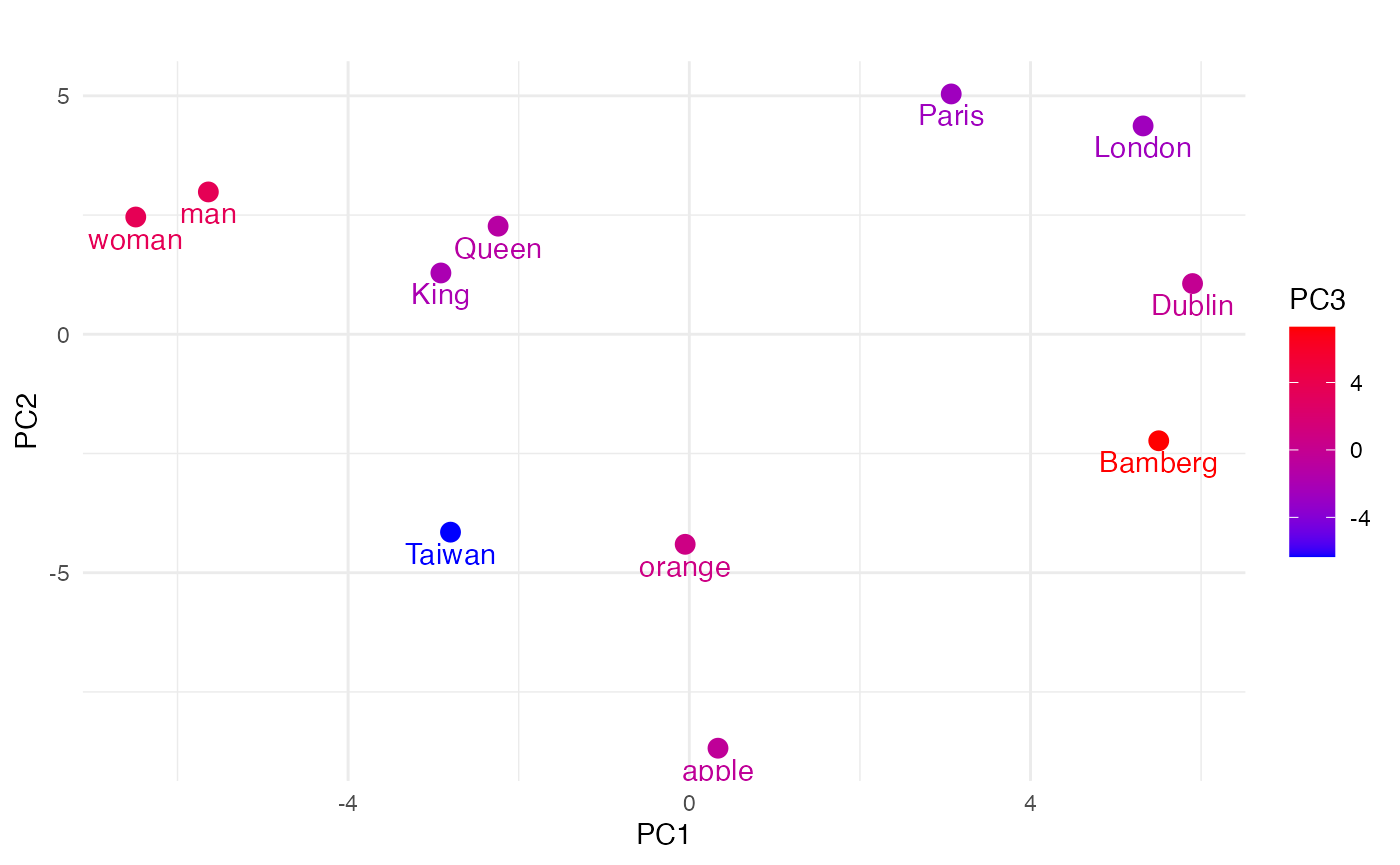
Stack Embeddings Method (GloVe + Back/forwad FlairEmbeddings or More)
# Initialize Embeddings -----------------------------
# Load embedding types from flaiR
WordEmbeddings <- flair_embeddings()$WordEmbeddings
FlairEmbeddings <- flair_embeddings()$FlairEmbeddings
StackedEmbeddings <- flair_embeddings()$StackedEmbeddings

# Configure Embeddings ----------------------------
# Initialize GloVe word embeddings
glove_embedding <- WordEmbeddings('glove')

# Initialize Flair contextual embeddings
flair_embedding_forward <- FlairEmbeddings('news-forward')
flair_embedding_backward <- FlairEmbeddings('news-backward')

# Initialize GloVe for individual use
embedding <- WordEmbeddings("glove")

# Create stacked embeddings combining GloVe and bidirectional Flair
stacked_embeddings <- StackedEmbeddings(c(glove_embedding,
                                         flair_embedding_forward,
                                         flair_embedding_backward))

# Text Processing --------------------------------
# Load Sentence class from flaiR
Sentence <- flair_data()$Sentence

# Create test sentence with semantic relationships
sentence <- Sentence("King Queen man woman Paris London apple orange Taiwan Dublin Bamberg")

# Apply embeddings and extract features ----------
# Embed text using stacked embeddings
stacked_embeddings$embed(sentence)

# Extract embeddings matrix with processing details
sen_df <- process_embeddings(sentence,
                           verbose = TRUE)
#> Extracting token embeddings...
#> Converting embeddings to matrix format...Processing completed in 0.004 seconds
#> Generated embedding matrix with 11 tokens and 4196 dimensions

# Dimensionality Reduction -----------------------
set.seed(123)

# Perform PCA for visualization
pca_result <- prcomp(sen_df, center = TRUE, scale. = TRUE)

# Extract first three principal components
word_embeddings_matrix <- as.data.frame(pca_result$x[,1:3])
word_embeddings_matrix
#>                PC1         PC2         PC3
#> King     -8.607464  67.2291073  32.4862897
#> Queen     1.757712  12.0477242 -26.8302591
#> man      70.603192  -6.6184846  13.1651727
#> woman    22.532037  -8.1126281  -0.9074069
#> Paris   -11.395620  -0.3051653 -17.5197047
#> London   -8.709174  -2.7450590 -14.1780509
#> apple    -8.739480 -15.7725165  -6.3796332
#> orange  -25.178335 -38.8501335  51.4907560
#> Taiwan   -9.132397  -5.0252071 -11.0918852
#> Dublin  -10.925014  -3.3407305 -10.1367702
#> Bamberg -12.205457   1.4930931 -10.0985081
# 2D Plot
library(ggplot2)

stacked_plot2D <- ggplot(word_embeddings_matrix, aes(x = PC1, y = PC2, color = PC3,
                                             label = rownames(word_embeddings_matrix))) +
  geom_point(size = 2) +
  geom_text(vjust = 1.5, hjust = 0.5) +
  scale_color_gradient(low = "blue", high = "red") +
  theme_minimal() +
  labs(title = "", x = "PC1", y = "PC2", color = "PC3")

stacked_plot2D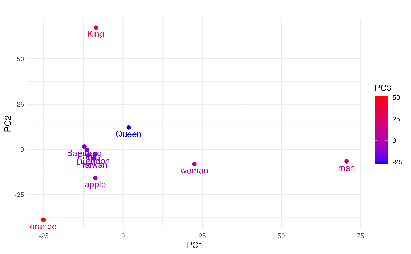
Transformer Embeddings (BERT or More)
# Load Required Package ----------------------------
library(flaiR)

# Initialize BERT and Text Processing --------------
# Import Sentence class for text operations
Sentence <- flair_data()$Sentence

# Initialize BERT model (base uncased version)
TransformerWordEmbeddings <- flair_embeddings()$TransformerWordEmbeddings("bert-base-uncased")

# Text Processing and Embedding --------------------
# Create sentence with semantic relationship pairs
sentence <- Sentence("King Queen man woman Paris London apple orange Taiwan Dublin Bamberg")

# Apply BERT embeddings to the sentence
TransformerWordEmbeddings$embed(sentence)
#> [[1]]
#> Sentence[11]: "King Queen man woman Paris London apple orange Taiwan Dublin Bamberg"

# Extract embeddings into matrix format
sen_df <- process_embeddings(sentence, verbose = TRUE)
#> Extracting token embeddings...
#> Converting embeddings to matrix format...Processing completed in 0.004 seconds
#> Generated embedding matrix with 11 tokens and 768 dimensions

# Dimensionality Reduction ------------------------
# Set random seed for reproducibility
set.seed(123)

# Apply PCA to reduce dimensions to 3 components
pca_result <- prcomp(sen_df, center = TRUE, scale. = TRUE)

# Extract first three principal components
word_embeddings_matrix <- as.data.frame(pca_result$x[,1:3])
word_embeddings_matrix
#>                 PC1        PC2        PC3
#> King    -11.6842542   4.264797  -2.539303
#> Queen   -18.6452604  13.278048  -9.781884
#> man     -18.3566181  10.571207  -1.609842
#> woman   -10.6397232  -2.072423   2.264132
#> Paris     6.9079152  -9.409334 -10.378022
#> London   10.7817678  -8.882271 -11.447016
#> apple    -0.6539754  -8.305123  12.104275
#> orange   -3.4409765  -4.756996  19.216482
#> Taiwan    4.5377967 -12.949604   4.782874
#> Dublin   13.4845075 -11.327307  -7.191567
#> Bamberg  27.7088205  29.589006   4.579870
# 2D Plot
library(ggplot2)

bert_plot2D <- ggplot(word_embeddings_matrix, aes(x = PC1, y = PC2, color = PC3,
                                             label = rownames(word_embeddings_matrix))) +
  geom_point(size = 2) +
  geom_text(vjust = 1.5, hjust = 0.5) +
  scale_color_gradient(low = "blue", high = "red") +
  theme_minimal() +
  labs(title = "", x = "PC1", y = "PC2", color = "PC3")
  # guides(color = "none")

stacked_plot2D
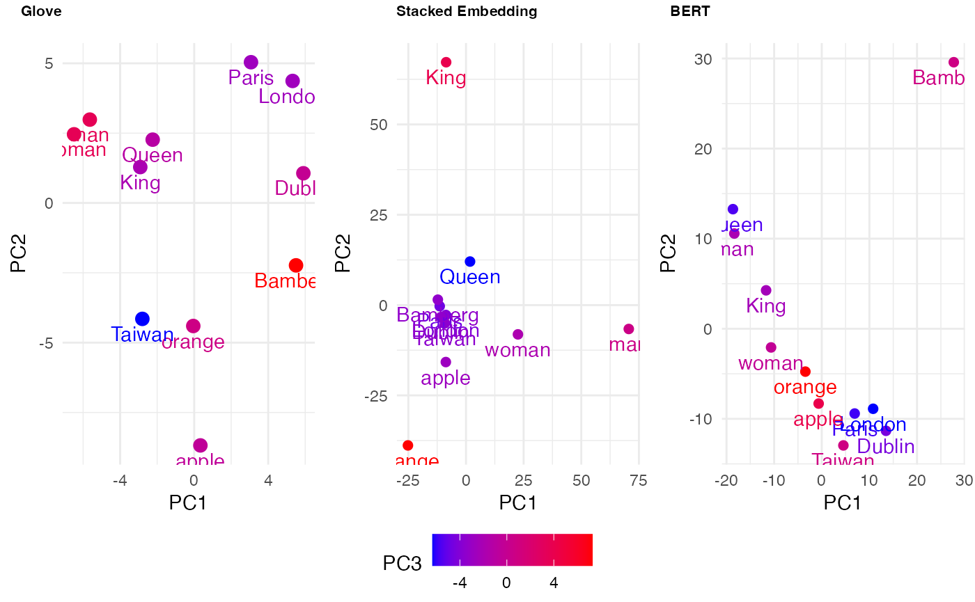
Training a Binary Classifier
In this section, we’ll train a sentiment analysis model that can categorize text as either positive or negative. This case study is adapted from pages 116 to 130 of Tadej Magajna’s book, ‘Natural Language Processing with Flair’. The process for training text classifiers in Flair mirrors the process followed for sequence labeling models. Specifically, the steps to train text classifiers are:
- Load a tagged corpus and compute the label dictionary map.
- Prepare the document embeddings.
- Initialize the
TextClassifierclass. - Train the model.
Loading a Tagged Corpus
Training text classification models requires a set of text documents (typically, sentences or paragraphs) where each document is associated with one or more classification labels. To train our sentiment analysis text classification model, we will be using the famous Internet Movie Database (IMDb) dataset, which contains 50,000 movie reviews from IMDB, where each review is labeled as either positive or negative. References to this dataset are already baked into Flair, so loading the dataset couldn’t be easier:
library(flaiR)
# load IMDB from flair_datasets module
Corpus <- flair_data()$Corpus
IMDB <- flair_datasets()$IMDB
# downsize to 0.05
corpus = IMDB()
#> 2025-10-29 01:22:58,768 Reading data from /Users/yenchiehliao/.flair/datasets/imdb_v4-rebalanced
#> 2025-10-29 01:22:58,769 Train: /Users/yenchiehliao/.flair/datasets/imdb_v4-rebalanced/train.txt
#> 2025-10-29 01:22:58,769 Dev: None
#> 2025-10-29 01:22:58,769 Test: None
#> 2025-10-29 01:22:59,379 No test split found. Using 10% (i.e. 5000 samples) of the train split as test data
#> 2025-10-29 01:22:59,395 No dev split found. Using 10% (i.e. 4500 samples) of the train split as dev data
#> 2025-10-29 01:22:59,395 Initialized corpus /Users/yenchiehliao/.flair/datasets/imdb_v4-rebalanced (label type name is 'sentiment')
corpus$downsample(0.05)
#> <flair.datasets.document_classification.IMDB object at 0x3e3743250>
Print the sizes in the corpus object as follows - test: %d | train: %d | dev: %d”
test_size <- length(corpus$test)
train_size <- length(corpus$train)
dev_size <- length(corpus$dev)
output <- sprintf("Corpus object sizes - Test: %d | Train: %d | Dev: %d", test_size, train_size, dev_size)
print(output)
#> [1] "Corpus object sizes - Test: 250 | Train: 2025 | Dev: 225"
lbl_type = 'sentiment'
label_dict = corpus$make_label_dictionary(label_type=lbl_type)
#> 2025-10-29 01:22:59,490 Computing label dictionary. Progress:
#> 2025-10-29 01:23:03,777 Dictionary created for label 'sentiment' with 2 values: POSITIVE (seen 1014 times), NEGATIVE (seen 1011 times)
Loading the Embeddings
flaiR covers all the different types of document embeddings that we
can use. Here, we simply use DocumentPoolEmbeddings. They
require no training prior to training the classification model
itself:
DocumentPoolEmbeddings <- flair_embeddings()$DocumentPoolEmbeddings
WordEmbeddings <- flair_embeddings()$WordEmbeddings
glove = WordEmbeddings('glove')
document_embeddings = DocumentPoolEmbeddings(glove)
Initializing the TextClassifier
# initiate TextClassifier
TextClassifier <- flair_models()$TextClassifier
classifier <- TextClassifier(document_embeddings,
                             label_dictionary = label_dict,
                             label_type = lbl_type)
$to allows you to set the device to use CPU, GPU, or
specific MPS devices on Mac (such as mps:0, mps:1, mps:2).
classifier$to(flair_device("mps")) TextClassifier(
(embeddings): DocumentPoolEmbeddings(
fine_tune_mode=none, pooling=mean
(embeddings): StackedEmbeddings(
(list_embedding_0): WordEmbeddings(
'glove'
(embedding): Embedding(400001, 100)
)
)
)
(decoder): Linear(in_features=100, out_features=3, bias=True)
(dropout): Dropout(p=0.0, inplace=False)
(locked_dropout): LockedDropout(p=0.0)
(word_dropout): WordDropout(p=0.0)
(loss_function): CrossEntropyLoss()
)Training the Model
Training the text classifier model involves two simple steps:
- Defining the model trainer class by passing in the classifier model and the corpus
- Setting off the training process passing in the required training hyper-parameters.
It is worth noting that the ‘L’ in numbers like 32L and 5L is used in R to denote that the number is an integer. Without the ‘L’ suffix, numbers in R are treated as numeric, which are by default double-precision floating-point numbers. In contrast, Python determines the type based on the value of the number itself. Whole numbers (e.g., 5 or 32) are of type int, while numbers with decimal points (e.g., 5.0) are of type float. Floating-point numbers in both languages are representations of real numbers but can have some approximation due to the way they are stored in memory.
# initiate ModelTrainer
ModelTrainer <- flair_trainers()$ModelTrainer

# fit the model
trainer <- ModelTrainer(classifier, corpus)

# start to train
# note: the 'L' in 32L is used in R to denote that the number is an integer.
trainer$train('classifier',
              learning_rate=0.1,
              mini_batch_size=32L,
              # specifies how embeddings are stored in RAM, ie."cpu", "cuda", "gpu", "mps".
              # embeddings_storage_mode = "mps",
              max_epochs=10L)
#> 2025-10-29 01:23:05,814 ----------------------------------------------------------------------------------------------------
#> 2025-10-29 01:23:05,814 Model: "TextClassifier(
#>   (embeddings): DocumentPoolEmbeddings(
#>     fine_tune_mode=none, pooling=mean
#>     (embeddings): StackedEmbeddings(
#>       (list_embedding_0): WordEmbeddings(
#>         'glove'
#>         (embedding): Embedding(400001, 100)
#>       )
#>     )
#>   )
#>   (decoder): Linear(in_features=100, out_features=2, bias=True)
#>   (dropout): Dropout(p=0.0, inplace=False)
#>   (locked_dropout): LockedDropout(p=0.0)
#>   (word_dropout): WordDropout(p=0.0)
#>   (loss_function): CrossEntropyLoss()
#>   (weights): None
#>   (weight_tensor) None
#> )"
#> 2025-10-29 01:23:05,814 ----------------------------------------------------------------------------------------------------
#> 2025-10-29 01:23:05,814 Corpus: 2025 train + 225 dev + 250 test sentences
#> 2025-10-29 01:23:05,814 ----------------------------------------------------------------------------------------------------
#> 2025-10-29 01:23:05,814 Train:  2025 sentences
#> 2025-10-29 01:23:05,814         (train_with_dev=False, train_with_test=False)
#> 2025-10-29 01:23:05,814 ----------------------------------------------------------------------------------------------------
#> 2025-10-29 01:23:05,814 Training Params:
#> 2025-10-29 01:23:05,814  - learning_rate: "0.1"
#> 2025-10-29 01:23:05,814  - mini_batch_size: "32"
#> 2025-10-29 01:23:05,814  - max_epochs: "10"
#> 2025-10-29 01:23:05,814  - shuffle: "True"
#> 2025-10-29 01:23:05,814 ----------------------------------------------------------------------------------------------------
#> 2025-10-29 01:23:05,814 Plugins:
#> 2025-10-29 01:23:05,815  - AnnealOnPlateau | patience: '3', anneal_factor: '0.5', min_learning_rate: '0.0001'
#> 2025-10-29 01:23:05,815 ----------------------------------------------------------------------------------------------------
#> 2025-10-29 01:23:05,815 Final evaluation on model from best epoch (best-model.pt)
#> 2025-10-29 01:23:05,815  - metric: "('micro avg', 'f1-score')"
#> 2025-10-29 01:23:05,815 ----------------------------------------------------------------------------------------------------
#> 2025-10-29 01:23:05,815 Computation:
#> 2025-10-29 01:23:05,815  - compute on device: cpu
#> 2025-10-29 01:23:05,815  - embedding storage: cpu
#> 2025-10-29 01:23:05,815 ----------------------------------------------------------------------------------------------------
#> 2025-10-29 01:23:05,815 Model training base path: "classifier"
#> 2025-10-29 01:23:05,815 ----------------------------------------------------------------------------------------------------
#> 2025-10-29 01:23:05,815 ----------------------------------------------------------------------------------------------------
#> 2025-10-29 01:23:06,770 epoch 1 - iter 6/64 - loss 1.03482102 - time (sec): 0.95 - samples/sec: 201.17 - lr: 0.100000 - momentum: 0.000000
#> 2025-10-29 01:23:07,682 epoch 1 - iter 12/64 - loss 0.97625112 - time (sec): 1.87 - samples/sec: 205.65 - lr: 0.100000 - momentum: 0.000000
#> 2025-10-29 01:23:08,524 epoch 1 - iter 18/64 - loss 0.97130605 - time (sec): 2.71 - samples/sec: 212.60 - lr: 0.100000 - momentum: 0.000000
#> 2025-10-29 01:23:09,433 epoch 1 - iter 24/64 - loss 0.96554917 - time (sec): 3.62 - samples/sec: 212.28 - lr: 0.100000 - momentum: 0.000000
#> 2025-10-29 01:23:10,296 epoch 1 - iter 30/64 - loss 0.95172536 - time (sec): 4.48 - samples/sec: 214.26 - lr: 0.100000 - momentum: 0.000000
#> 2025-10-29 01:23:11,127 epoch 1 - iter 36/64 - loss 0.93596985 - time (sec): 5.31 - samples/sec: 216.88 - lr: 0.100000 - momentum: 0.000000
#> 2025-10-29 01:23:12,096 epoch 1 - iter 42/64 - loss 0.93621534 - time (sec): 6.28 - samples/sec: 213.99 - lr: 0.100000 - momentum: 0.000000
#> 2025-10-29 01:23:13,066 epoch 1 - iter 48/64 - loss 0.93329721 - time (sec): 7.25 - samples/sec: 211.85 - lr: 0.100000 - momentum: 0.000000
#> 2025-10-29 01:23:14,161 epoch 1 - iter 54/64 - loss 0.92732978 - time (sec): 8.35 - samples/sec: 207.05 - lr: 0.100000 - momentum: 0.000000
#> 2025-10-29 01:23:15,065 epoch 1 - iter 60/64 - loss 0.91905521 - time (sec): 9.25 - samples/sec: 207.58 - lr: 0.100000 - momentum: 0.000000
#> 2025-10-29 01:23:15,565 ----------------------------------------------------------------------------------------------------
#> 2025-10-29 01:23:15,565 EPOCH 1 done: loss 0.9183 - lr: 0.100000
#> 2025-10-29 01:23:16,665 DEV : loss 0.969170331954956 - f1-score (micro avg)  0.4533
#> 2025-10-29 01:23:17,349  - 0 epochs without improvement
#> 2025-10-29 01:23:17,351 saving best model
#> 2025-10-29 01:23:17,796 ----------------------------------------------------------------------------------------------------
#> 2025-10-29 01:23:18,713 epoch 2 - iter 6/64 - loss 0.89565008 - time (sec): 0.92 - samples/sec: 209.50 - lr: 0.100000 - momentum: 0.000000
#> 2025-10-29 01:23:19,564 epoch 2 - iter 12/64 - loss 0.91454447 - time (sec): 1.77 - samples/sec: 217.32 - lr: 0.100000 - momentum: 0.000000
#> 2025-10-29 01:23:20,364 epoch 2 - iter 18/64 - loss 0.87032511 - time (sec): 2.57 - samples/sec: 224.41 - lr: 0.100000 - momentum: 0.000000
#> 2025-10-29 01:23:21,176 epoch 2 - iter 24/64 - loss 0.89476166 - time (sec): 3.38 - samples/sec: 227.27 - lr: 0.100000 - momentum: 0.000000
#> 2025-10-29 01:23:22,017 epoch 2 - iter 30/64 - loss 0.89790537 - time (sec): 4.22 - samples/sec: 227.49 - lr: 0.100000 - momentum: 0.000000
#> 2025-10-29 01:23:22,806 epoch 2 - iter 36/64 - loss 0.88154723 - time (sec): 5.01 - samples/sec: 229.96 - lr: 0.100000 - momentum: 0.000000
#> 2025-10-29 01:23:23,643 epoch 2 - iter 42/64 - loss 0.89160718 - time (sec): 5.85 - samples/sec: 229.89 - lr: 0.100000 - momentum: 0.000000
#> 2025-10-29 01:23:24,725 epoch 2 - iter 48/64 - loss 0.88830253 - time (sec): 6.93 - samples/sec: 221.70 - lr: 0.100000 - momentum: 0.000000
#> 2025-10-29 01:23:25,520 epoch 2 - iter 54/64 - loss 0.88188778 - time (sec): 7.72 - samples/sec: 223.75 - lr: 0.100000 - momentum: 0.000000
#> 2025-10-29 01:23:26,273 epoch 2 - iter 60/64 - loss 0.87024007 - time (sec): 8.48 - samples/sec: 226.52 - lr: 0.100000 - momentum: 0.000000
#> 2025-10-29 01:23:26,604 ----------------------------------------------------------------------------------------------------
#> 2025-10-29 01:23:26,604 EPOCH 2 done: loss 0.8670 - lr: 0.100000
#> 2025-10-29 01:23:27,857 DEV : loss 0.6613298654556274 - f1-score (micro avg)  0.56
#> 2025-10-29 01:23:28,315  - 0 epochs without improvement
#> 2025-10-29 01:23:28,318 saving best model
#> 2025-10-29 01:23:28,661 ----------------------------------------------------------------------------------------------------
#> 2025-10-29 01:23:29,508 epoch 3 - iter 6/64 - loss 0.97559432 - time (sec): 0.85 - samples/sec: 226.91 - lr: 0.100000 - momentum: 0.000000
#> 2025-10-29 01:23:30,322 epoch 3 - iter 12/64 - loss 0.96988676 - time (sec): 1.66 - samples/sec: 231.23 - lr: 0.100000 - momentum: 0.000000
#> 2025-10-29 01:23:31,389 epoch 3 - iter 18/64 - loss 0.95166033 - time (sec): 2.73 - samples/sec: 211.17 - lr: 0.100000 - momentum: 0.000000
#> 2025-10-29 01:23:32,115 epoch 3 - iter 24/64 - loss 0.94594647 - time (sec): 3.45 - samples/sec: 222.37 - lr: 0.100000 - momentum: 0.000000
#> 2025-10-29 01:23:32,920 epoch 3 - iter 30/64 - loss 0.92877954 - time (sec): 4.26 - samples/sec: 225.42 - lr: 0.100000 - momentum: 0.000000
#> 2025-10-29 01:23:33,762 epoch 3 - iter 36/64 - loss 0.90791758 - time (sec): 5.10 - samples/sec: 225.84 - lr: 0.100000 - momentum: 0.000000
#> 2025-10-29 01:23:34,587 epoch 3 - iter 42/64 - loss 0.90284721 - time (sec): 5.93 - samples/sec: 226.81 - lr: 0.100000 - momentum: 0.000000
#> 2025-10-29 01:23:35,494 epoch 3 - iter 48/64 - loss 0.89997107 - time (sec): 6.83 - samples/sec: 224.79 - lr: 0.100000 - momentum: 0.000000
#> 2025-10-29 01:23:36,305 epoch 3 - iter 54/64 - loss 0.89072626 - time (sec): 7.64 - samples/sec: 226.07 - lr: 0.100000 - momentum: 0.000000
#> 2025-10-29 01:23:37,170 epoch 3 - iter 60/64 - loss 0.89468155 - time (sec): 8.51 - samples/sec: 225.64 - lr: 0.100000 - momentum: 0.000000
#> 2025-10-29 01:23:37,681 ----------------------------------------------------------------------------------------------------
#> 2025-10-29 01:23:37,681 EPOCH 3 done: loss 0.8853 - lr: 0.100000
#> 2025-10-29 01:23:38,739 DEV : loss 0.9235679507255554 - f1-score (micro avg)  0.4533
#> 2025-10-29 01:23:39,488  - 1 epochs without improvement
#> 2025-10-29 01:23:39,490 ----------------------------------------------------------------------------------------------------
#> 2025-10-29 01:23:40,352 epoch 4 - iter 6/64 - loss 0.82624254 - time (sec): 0.86 - samples/sec: 222.81 - lr: 0.100000 - momentum: 0.000000
#> 2025-10-29 01:23:41,155 epoch 4 - iter 12/64 - loss 0.90411119 - time (sec): 1.66 - samples/sec: 230.74 - lr: 0.100000 - momentum: 0.000000
#> 2025-10-29 01:23:42,076 epoch 4 - iter 18/64 - loss 0.85366339 - time (sec): 2.59 - samples/sec: 222.79 - lr: 0.100000 - momentum: 0.000000
#> 2025-10-29 01:23:42,900 epoch 4 - iter 24/64 - loss 0.83558531 - time (sec): 3.41 - samples/sec: 225.26 - lr: 0.100000 - momentum: 0.000000
#> 2025-10-29 01:23:43,698 epoch 4 - iter 30/64 - loss 0.85402448 - time (sec): 4.21 - samples/sec: 228.16 - lr: 0.100000 - momentum: 0.000000
#> 2025-10-29 01:23:44,658 epoch 4 - iter 36/64 - loss 0.85074003 - time (sec): 5.17 - samples/sec: 222.93 - lr: 0.100000 - momentum: 0.000000
#> 2025-10-29 01:23:45,493 epoch 4 - iter 42/64 - loss 0.83589199 - time (sec): 6.00 - samples/sec: 223.91 - lr: 0.100000 - momentum: 0.000000
#> 2025-10-29 01:23:46,316 epoch 4 - iter 48/64 - loss 0.84322071 - time (sec): 6.83 - samples/sec: 225.03 - lr: 0.100000 - momentum: 0.000000
#> 2025-10-29 01:23:47,048 epoch 4 - iter 54/64 - loss 0.83743314 - time (sec): 7.56 - samples/sec: 228.63 - lr: 0.100000 - momentum: 0.000000
#> 2025-10-29 01:23:47,842 epoch 4 - iter 60/64 - loss 0.83712479 - time (sec): 8.35 - samples/sec: 229.90 - lr: 0.100000 - momentum: 0.000000
#> 2025-10-29 01:23:48,357 ----------------------------------------------------------------------------------------------------
#> 2025-10-29 01:23:48,357 EPOCH 4 done: loss 0.8385 - lr: 0.100000
#> 2025-10-29 01:23:49,395 DEV : loss 0.902965784072876 - f1-score (micro avg)  0.4533
#> 2025-10-29 01:23:50,087  - 2 epochs without improvement
#> 2025-10-29 01:23:50,089 ----------------------------------------------------------------------------------------------------
#> 2025-10-29 01:23:50,877 epoch 5 - iter 6/64 - loss 0.83386131 - time (sec): 0.79 - samples/sec: 243.70 - lr: 0.100000 - momentum: 0.000000
#> 2025-10-29 01:23:51,643 epoch 5 - iter 12/64 - loss 0.81110337 - time (sec): 1.55 - samples/sec: 247.09 - lr: 0.100000 - momentum: 0.000000
#> 2025-10-29 01:23:52,448 epoch 5 - iter 18/64 - loss 0.81918713 - time (sec): 2.36 - samples/sec: 244.19 - lr: 0.100000 - momentum: 0.000000
#> 2025-10-29 01:23:53,246 epoch 5 - iter 24/64 - loss 0.82163843 - time (sec): 3.16 - samples/sec: 243.23 - lr: 0.100000 - momentum: 0.000000
#> 2025-10-29 01:23:54,060 epoch 5 - iter 30/64 - loss 0.80355368 - time (sec): 3.97 - samples/sec: 241.72 - lr: 0.100000 - momentum: 0.000000
#> 2025-10-29 01:23:54,888 epoch 5 - iter 36/64 - loss 0.82123225 - time (sec): 4.80 - samples/sec: 240.03 - lr: 0.100000 - momentum: 0.000000
#> 2025-10-29 01:23:55,656 epoch 5 - iter 42/64 - loss 0.83147700 - time (sec): 5.57 - samples/sec: 241.39 - lr: 0.100000 - momentum: 0.000000
#> 2025-10-29 01:23:56,605 epoch 5 - iter 48/64 - loss 0.82776047 - time (sec): 6.52 - samples/sec: 235.74 - lr: 0.100000 - momentum: 0.000000
#> 2025-10-29 01:23:57,375 epoch 5 - iter 54/64 - loss 0.82137293 - time (sec): 7.29 - samples/sec: 237.16 - lr: 0.100000 - momentum: 0.000000
#> 2025-10-29 01:23:58,180 epoch 5 - iter 60/64 - loss 0.82507927 - time (sec): 8.09 - samples/sec: 237.30 - lr: 0.100000 - momentum: 0.000000
#> 2025-10-29 01:23:58,554 ----------------------------------------------------------------------------------------------------
#> 2025-10-29 01:23:58,554 EPOCH 5 done: loss 0.8266 - lr: 0.100000
#> 2025-10-29 01:23:59,796 DEV : loss 0.8814549446105957 - f1-score (micro avg)  0.4533
#> 2025-10-29 01:24:00,273  - 3 epochs without improvement
#> 2025-10-29 01:24:00,275 ----------------------------------------------------------------------------------------------------
#> 2025-10-29 01:24:01,355 epoch 6 - iter 6/64 - loss 0.86599507 - time (sec): 1.08 - samples/sec: 177.86 - lr: 0.100000 - momentum: 0.000000
#> 2025-10-29 01:24:02,147 epoch 6 - iter 12/64 - loss 0.83119471 - time (sec): 1.87 - samples/sec: 205.21 - lr: 0.100000 - momentum: 0.000000
#> 2025-10-29 01:24:02,930 epoch 6 - iter 18/64 - loss 0.83965523 - time (sec): 2.65 - samples/sec: 217.00 - lr: 0.100000 - momentum: 0.000000
#> 2025-10-29 01:24:03,696 epoch 6 - iter 24/64 - loss 0.82790930 - time (sec): 3.42 - samples/sec: 224.54 - lr: 0.100000 - momentum: 0.000000
#> 2025-10-29 01:24:04,455 epoch 6 - iter 30/64 - loss 0.82493706 - time (sec): 4.18 - samples/sec: 229.70 - lr: 0.100000 - momentum: 0.000000
#> 2025-10-29 01:24:05,286 epoch 6 - iter 36/64 - loss 0.82221150 - time (sec): 5.01 - samples/sec: 229.91 - lr: 0.100000 - momentum: 0.000000
#> 2025-10-29 01:24:06,080 epoch 6 - iter 42/64 - loss 0.82115991 - time (sec): 5.80 - samples/sec: 231.56 - lr: 0.100000 - momentum: 0.000000
#> 2025-10-29 01:24:06,867 epoch 6 - iter 48/64 - loss 0.82263479 - time (sec): 6.59 - samples/sec: 233.04 - lr: 0.100000 - momentum: 0.000000
#> 2025-10-29 01:24:07,616 epoch 6 - iter 54/64 - loss 0.81930931 - time (sec): 7.34 - samples/sec: 235.41 - lr: 0.100000 - momentum: 0.000000
#> 2025-10-29 01:24:08,577 epoch 6 - iter 60/64 - loss 0.81072097 - time (sec): 8.30 - samples/sec: 231.29 - lr: 0.100000 - momentum: 0.000000
#> 2025-10-29 01:24:08,931 ----------------------------------------------------------------------------------------------------
#> 2025-10-29 01:24:08,931 EPOCH 6 done: loss 0.8158 - lr: 0.100000
#> 2025-10-29 01:24:10,022 DEV : loss 0.7792848944664001 - f1-score (micro avg)  0.5556
#> 2025-10-29 01:24:10,730  - 4 epochs without improvement (above 'patience')-> annealing learning_rate to [0.05]
#> 2025-10-29 01:24:10,732 ----------------------------------------------------------------------------------------------------
#> 2025-10-29 01:24:11,539 epoch 7 - iter 6/64 - loss 0.62141190 - time (sec): 0.81 - samples/sec: 237.97 - lr: 0.050000 - momentum: 0.000000
#> 2025-10-29 01:24:12,333 epoch 7 - iter 12/64 - loss 0.60887330 - time (sec): 1.60 - samples/sec: 239.91 - lr: 0.050000 - momentum: 0.000000
#> 2025-10-29 01:24:13,096 epoch 7 - iter 18/64 - loss 0.60901921 - time (sec): 2.36 - samples/sec: 243.75 - lr: 0.050000 - momentum: 0.000000
#> 2025-10-29 01:24:13,860 epoch 7 - iter 24/64 - loss 0.62312240 - time (sec): 3.13 - samples/sec: 245.53 - lr: 0.050000 - momentum: 0.000000
#> 2025-10-29 01:24:14,832 epoch 7 - iter 30/64 - loss 0.64444851 - time (sec): 4.10 - samples/sec: 234.18 - lr: 0.050000 - momentum: 0.000000
#> 2025-10-29 01:24:15,608 epoch 7 - iter 36/64 - loss 0.64126529 - time (sec): 4.88 - samples/sec: 236.27 - lr: 0.050000 - momentum: 0.000000
#> 2025-10-29 01:24:16,393 epoch 7 - iter 42/64 - loss 0.65158008 - time (sec): 5.66 - samples/sec: 237.43 - lr: 0.050000 - momentum: 0.000000
#> 2025-10-29 01:24:17,197 epoch 7 - iter 48/64 - loss 0.65823784 - time (sec): 6.47 - samples/sec: 237.59 - lr: 0.050000 - momentum: 0.000000
#> 2025-10-29 01:24:18,004 epoch 7 - iter 54/64 - loss 0.65939955 - time (sec): 7.27 - samples/sec: 237.64 - lr: 0.050000 - momentum: 0.000000
#> 2025-10-29 01:24:18,855 epoch 7 - iter 60/64 - loss 0.66072118 - time (sec): 8.12 - samples/sec: 236.37 - lr: 0.050000 - momentum: 0.000000
#> 2025-10-29 01:24:19,424 ----------------------------------------------------------------------------------------------------
#> 2025-10-29 01:24:19,425 EPOCH 7 done: loss 0.6589 - lr: 0.050000
#> 2025-10-29 01:24:20,492 DEV : loss 0.6003721356391907 - f1-score (micro avg)  0.6978
#> 2025-10-29 01:24:21,203  - 0 epochs without improvement
#> 2025-10-29 01:24:21,205 saving best model
#> 2025-10-29 01:24:21,548 ----------------------------------------------------------------------------------------------------
#> 2025-10-29 01:24:22,373 epoch 8 - iter 6/64 - loss 0.65252212 - time (sec): 0.82 - samples/sec: 232.88 - lr: 0.050000 - momentum: 0.000000
#> 2025-10-29 01:24:23,196 epoch 8 - iter 12/64 - loss 0.63390189 - time (sec): 1.65 - samples/sec: 233.08 - lr: 0.050000 - momentum: 0.000000
#> 2025-10-29 01:24:23,977 epoch 8 - iter 18/64 - loss 0.63412659 - time (sec): 2.43 - samples/sec: 237.13 - lr: 0.050000 - momentum: 0.000000
#> 2025-10-29 01:24:24,767 epoch 8 - iter 24/64 - loss 0.63389341 - time (sec): 3.22 - samples/sec: 238.61 - lr: 0.050000 - momentum: 0.000000
#> 2025-10-29 01:24:25,561 epoch 8 - iter 30/64 - loss 0.63322895 - time (sec): 4.01 - samples/sec: 239.26 - lr: 0.050000 - momentum: 0.000000
#> 2025-10-29 01:24:26,578 epoch 8 - iter 36/64 - loss 0.63415459 - time (sec): 5.03 - samples/sec: 229.02 - lr: 0.050000 - momentum: 0.000000
#> 2025-10-29 01:24:27,403 epoch 8 - iter 42/64 - loss 0.63968469 - time (sec): 5.85 - samples/sec: 229.58 - lr: 0.050000 - momentum: 0.000000
#> 2025-10-29 01:24:28,177 epoch 8 - iter 48/64 - loss 0.65097602 - time (sec): 6.63 - samples/sec: 231.71 - lr: 0.050000 - momentum: 0.000000
#> 2025-10-29 01:24:29,000 epoch 8 - iter 54/64 - loss 0.65496666 - time (sec): 7.45 - samples/sec: 231.89 - lr: 0.050000 - momentum: 0.000000
#> 2025-10-29 01:24:29,887 epoch 8 - iter 60/64 - loss 0.64874915 - time (sec): 8.34 - samples/sec: 230.26 - lr: 0.050000 - momentum: 0.000000
#> 2025-10-29 01:24:30,469 ----------------------------------------------------------------------------------------------------
#> 2025-10-29 01:24:30,469 EPOCH 8 done: loss 0.6494 - lr: 0.050000
#> 2025-10-29 01:24:31,624 DEV : loss 0.6876248717308044 - f1-score (micro avg)  0.5467
#> 2025-10-29 01:24:32,363  - 1 epochs without improvement
#> 2025-10-29 01:24:32,365 ----------------------------------------------------------------------------------------------------
#> 2025-10-29 01:24:33,265 epoch 9 - iter 6/64 - loss 0.64467014 - time (sec): 0.90 - samples/sec: 213.27 - lr: 0.050000 - momentum: 0.000000
#> 2025-10-29 01:24:34,160 epoch 9 - iter 12/64 - loss 0.64915569 - time (sec): 1.80 - samples/sec: 213.88 - lr: 0.050000 - momentum: 0.000000
#> 2025-10-29 01:24:35,019 epoch 9 - iter 18/64 - loss 0.63960192 - time (sec): 2.65 - samples/sec: 217.07 - lr: 0.050000 - momentum: 0.000000
#> 2025-10-29 01:24:35,991 epoch 9 - iter 24/64 - loss 0.62827631 - time (sec): 3.63 - samples/sec: 211.81 - lr: 0.050000 - momentum: 0.000000
#> 2025-10-29 01:24:36,903 epoch 9 - iter 30/64 - loss 0.63651646 - time (sec): 4.54 - samples/sec: 211.53 - lr: 0.050000 - momentum: 0.000000
#> 2025-10-29 01:24:37,671 epoch 9 - iter 36/64 - loss 0.63269677 - time (sec): 5.31 - samples/sec: 217.11 - lr: 0.050000 - momentum: 0.000000
#> 2025-10-29 01:24:38,433 epoch 9 - iter 42/64 - loss 0.64019648 - time (sec): 6.07 - samples/sec: 221.47 - lr: 0.050000 - momentum: 0.000000
#> 2025-10-29 01:24:39,413 epoch 9 - iter 48/64 - loss 0.64170534 - time (sec): 7.05 - samples/sec: 217.94 - lr: 0.050000 - momentum: 0.000000
#> 2025-10-29 01:24:40,240 epoch 9 - iter 54/64 - loss 0.63846545 - time (sec): 7.88 - samples/sec: 219.42 - lr: 0.050000 - momentum: 0.000000
#> 2025-10-29 01:24:41,278 epoch 9 - iter 60/64 - loss 0.63938779 - time (sec): 8.91 - samples/sec: 215.41 - lr: 0.050000 - momentum: 0.000000
#> 2025-10-29 01:24:41,617 ----------------------------------------------------------------------------------------------------
#> 2025-10-29 01:24:41,618 EPOCH 9 done: loss 0.6397 - lr: 0.050000
#> 2025-10-29 01:24:42,726 DEV : loss 0.5814307332038879 - f1-score (micro avg)  0.7156
#> 2025-10-29 01:24:43,459  - 0 epochs without improvement
#> 2025-10-29 01:24:43,463 saving best model
#> 2025-10-29 01:24:43,816 ----------------------------------------------------------------------------------------------------
#> 2025-10-29 01:24:44,652 epoch 10 - iter 6/64 - loss 0.60317001 - time (sec): 0.84 - samples/sec: 229.69 - lr: 0.050000 - momentum: 0.000000
#> 2025-10-29 01:24:45,509 epoch 10 - iter 12/64 - loss 0.61682722 - time (sec): 1.69 - samples/sec: 226.77 - lr: 0.050000 - momentum: 0.000000
#> 2025-10-29 01:24:46,544 epoch 10 - iter 18/64 - loss 0.61251386 - time (sec): 2.73 - samples/sec: 211.16 - lr: 0.050000 - momentum: 0.000000
#> 2025-10-29 01:24:47,391 epoch 10 - iter 24/64 - loss 0.61089186 - time (sec): 3.57 - samples/sec: 214.83 - lr: 0.050000 - momentum: 0.000000
#> 2025-10-29 01:24:48,294 epoch 10 - iter 30/64 - loss 0.62348493 - time (sec): 4.48 - samples/sec: 214.40 - lr: 0.050000 - momentum: 0.000000
#> 2025-10-29 01:24:49,103 epoch 10 - iter 36/64 - loss 0.61944086 - time (sec): 5.29 - samples/sec: 217.88 - lr: 0.050000 - momentum: 0.000000
#> 2025-10-29 01:24:49,954 epoch 10 - iter 42/64 - loss 0.62064590 - time (sec): 6.14 - samples/sec: 218.96 - lr: 0.050000 - momentum: 0.000000
#> 2025-10-29 01:24:50,803 epoch 10 - iter 48/64 - loss 0.62229136 - time (sec): 6.99 - samples/sec: 219.85 - lr: 0.050000 - momentum: 0.000000
#> 2025-10-29 01:24:51,662 epoch 10 - iter 54/64 - loss 0.62610477 - time (sec): 7.85 - samples/sec: 220.26 - lr: 0.050000 - momentum: 0.000000
#> 2025-10-29 01:24:52,467 epoch 10 - iter 60/64 - loss 0.62748551 - time (sec): 8.65 - samples/sec: 221.94 - lr: 0.050000 - momentum: 0.000000
#> 2025-10-29 01:24:53,012 ----------------------------------------------------------------------------------------------------
#> 2025-10-29 01:24:53,013 EPOCH 10 done: loss 0.6305 - lr: 0.050000
#> 2025-10-29 01:24:54,189 DEV : loss 0.5568863153457642 - f1-score (micro avg)  0.7244
#> 2025-10-29 01:24:54,901  - 0 epochs without improvement
#> 2025-10-29 01:24:54,903 saving best model
#> 2025-10-29 01:24:55,728 ----------------------------------------------------------------------------------------------------
#> 2025-10-29 01:24:55,728 Loading model from best epoch ...
#> 2025-10-29 01:24:57,453
#> Results:
#> - F-score (micro) 0.712
#> - F-score (macro) 0.7078
#> - Accuracy 0.712
#>
#> By class:
#>               precision    recall  f1-score   support
#>
#>     NEGATIVE     0.6541    0.8595    0.7429       121
#>     POSITIVE     0.8132    0.5736    0.6727       129
#>
#>     accuracy                         0.7120       250
#>    macro avg     0.7336    0.7166    0.7078       250
#> weighted avg     0.7362    0.7120    0.7067       250
#>
#> 2025-10-29 01:24:57,453 ----------------------------------------------------------------------------------------------------
#> $test_score
#> [1] 0.712
Loading and Using the Classifiers
After training the text classification model, the resulting classifier will already be stored in memory as part of the classifier variable. It is possible, however, that your Python session exited after training. If so, you’ll need to load the model into memory with the following:
TextClassifier <- flair_models()$TextClassifier
classifier <- TextClassifier$load('classifier/best-model.pt')
We import the Sentence object. Now, we can generate predictions on some example text inputs.
Sentence <- flair_data()$Sentence
sentence <- Sentence("great")
classifier$predict(sentence)
print(sentence$labels)
#> [[1]]
#> 'Sentence[1]: "great"'/'POSITIVE' (1.0)
sentence <- Sentence("sad")
classifier$predict(sentence)
print(sentence$labels)
#> [[1]]
#> 'Sentence[1]: "sad"'/'NEGATIVE' (0.6663)
Training RNNs
Here, we train a sentiment analysis model to categorize text. In this case, we also include a pipeline that implements the use of Recurrent Neural Networks (RNN). This makes them particularly effective for tasks involving sequential data. This section also show you how to implement one of most powerful features in flaiR, stacked embeddings. You can stack multiple embeddings with different layers and let the classifier learn from different types of features. In Flair NLP, and with the flaiR package, it’s very easy to accomplish this task.
Import Necessary Modules
library(flaiR)
WordEmbeddings <- flair_embeddings()$WordEmbeddings
FlairEmbeddings <- flair_embeddings()$FlairEmbeddings
DocumentRNNEmbeddings <- flair_embeddings()$DocumentRNNEmbeddings
TextClassifier <- flair_models()$TextClassifier
ModelTrainer <- flair_trainers()$ModelTrainer
Get the IMDB Corpus
The IMDB movie review dataset is used here, which is a commonly
utilized dataset for sentiment analysis. $downsample(0.1)
method means only 10% of the dataset is used, allowing for a faster
demonstration.
# load the IMDB file and downsize it to 0.1
IMDB <- flair_datasets()$IMDB
corpus <- IMDB()$downsample(0.1)
#> 2025-10-29 01:24:57,892 Reading data from /Users/yenchiehliao/.flair/datasets/imdb_v4-rebalanced
#> 2025-10-29 01:24:57,892 Train: /Users/yenchiehliao/.flair/datasets/imdb_v4-rebalanced/train.txt
#> 2025-10-29 01:24:57,892 Dev: None
#> 2025-10-29 01:24:57,892 Test: None
#> 2025-10-29 01:24:58,471 No test split found. Using 10% (i.e. 5000 samples) of the train split as test data
#> 2025-10-29 01:24:58,487 No dev split found. Using 10% (i.e. 4500 samples) of the train split as dev data
#> 2025-10-29 01:24:58,487 Initialized corpus /Users/yenchiehliao/.flair/datasets/imdb_v4-rebalanced (label type name is 'sentiment')
# create the label dictionary
lbl_type <- 'sentiment'
label_dict <- corpus$make_label_dictionary(label_type=lbl_type)
#> 2025-10-29 01:24:58,504 Computing label dictionary. Progress:
#> 2025-10-29 01:25:06,982 Dictionary created for label 'sentiment' with 2 values: POSITIVE (seen 2056 times), NEGATIVE (seen 1994 times)
Stacked Embeddings
This is one of Flair’s most powerful features: it allows for the integration of embeddings to enable the model to learn from more sparse features. Three types of embeddings are utilized here: GloVe embeddings, and two types of Flair embeddings (forward and backward). Word embeddings are used to convert words into vectors.
# make a list of word embeddings
word_embeddings <- list(WordEmbeddings('glove'),
                        FlairEmbeddings('news-forward-fast'),
                        FlairEmbeddings('news-backward-fast'))

# initialize the document embeddings
document_embeddings <- DocumentRNNEmbeddings(word_embeddings,
                                             hidden_size = 512L,
                                             reproject_words = TRUE,
                                             reproject_words_dimension = 256L)
# create a Text Classifier with the embeddings and label dictionary
classifier <- TextClassifier(document_embeddings,
                            label_dictionary=label_dict, label_type='class')

# initialize the text classifier trainer with our corpus
trainer <- ModelTrainer(classifier, corpus)
Start the Training
For the sake of this example, setting max_epochs to 5. You might want to increase this for better performance.
It is worth noting that the learning rate is a parameter that
determines the step size at each iteration while moving towards a
minimum of the loss function. A smaller learning rate could slow down
the learning process, but it could lead to more precise convergence.
mini_batch_size determines the number of samples that will
be used to compute the gradient at each step. The ‘L’ in 32L is used in
R to denote that the number is an integer.
patience (aka early stop) is a hyper-parameter used in
conjunction with early stopping to avoid overfitting. It determines the
number of epochs the training process will tolerate without improvements
before stopping the training. Setting max_epochs to 5 means the
algorithm will make five passes through the dataset.
# note: the 'L' in 32L is used in R to denote that the number is an integer.
trainer$train('models/sentiment',
              learning_rate=0.1,
              mini_batch_size=32L,
              patience=5L,
              max_epochs=5L)
To Apply the Trained Model for Prediction
sentence <- "This movie was really exciting!"
classifier$predict(sentence)
print(sentence.labels)
Finetune Transformers
We use data from The Temporal Focus of Campaign Communication
(2020 JOP) as an example. Let’s assume we receive the data for
training from different times. First, suppose you have a dataset of 1000
entries called cc_muller_old. On another day, with the help
of nice friends, you receive another set of data, adding 2000 entries in
a dataset called cc_muller_new. Both subsets are from
data(cc_muller). We will show how to fine-tune a
transformer model with cc_muller_old, and then continue
with another round of fine-tuning using cc_muller_new.
Fine-tuning a Transformers Model
Step 1 Load Necessary Modules from Flair
Load necessary classes from flair package.
# Sentence is a class for holding a text sentence
Sentence <- flair_data()$Sentence

# Corpus is a class for text corpora
Corpus <- flair_data()$Corpus

# TransformerDocumentEmbeddings is a class for loading transformer
TransformerDocumentEmbeddings <- flair_embeddings()$TransformerDocumentEmbeddings

# TextClassifier is a class for text classification
TextClassifier <- flair_models()$TextClassifier

# ModelTrainer is a class for training and evaluating models
ModelTrainer <- flair_trainers()$ModelTrainer
We use purrr to help us split sentences using Sentence from
flair_data(), then use map2 to add labels, and finally use
Corpus to segment the data.
library(purrr)

data(cc_muller)
cc_muller_old <- cc_muller[1:1000,]

old_text <- map(cc_muller_old$text, Sentence)
old_labels <- as.character(cc_muller_old$class)

old_text <- map2(old_text, old_labels, ~ {
  .x$add_label("classification", .y)
  .x
})
set.seed(2046)
sample <- sample(c(TRUE, FALSE), length(old_text), replace=TRUE, prob=c(0.8, 0.2))
old_train  <- old_text[sample]
old_test   <- old_text[!sample]

test_id <- sample(c(TRUE, FALSE), length(old_test), replace=TRUE, prob=c(0.5, 0.5))
old_test   <- old_test[test_id]
old_dev   <- old_test[!test_id]
If you do not provide a development set (dev set) while using Flair, it will automatically split the training data into training and development datasets. The test set is used for training the model and evaluating its final performance, whereas the development set is used for adjusting model parameters and preventing overfitting, or in other words, for early stopping of the model.
old_corpus <- Corpus(train = old_train, test = old_test)
#> 2025-10-29 01:25:09,286 No dev split found. Using 10% (i.e. 80 samples) of the train split as dev data
Step 3 Load distilbert
Transformer
document_embeddings <- TransformerDocumentEmbeddings('distilbert-base-uncased', fine_tune=TRUE)First, the $make_label_dictionary function is used to
automatically create a label dictionary for the classification task. The
label dictionary is a mapping from label to index, which is used to map
the labels to a tensor of label indices. Besides classification tasks,
flaiR also supports other label types for training custom model. From
the cc_muller dataset: Future (seen 423 times), Present (seen 262
times), Past (seen 131 times).
old_label_dict <- old_corpus$make_label_dictionary(label_type="classification")
#> 2025-10-29 01:25:10,398 Computing label dictionary. Progress:
#> 2025-10-29 01:25:10,407 Dictionary created for label 'classification' with 3 values: Future (seen 380 times), Present (seen 232 times), Past (seen 111 times)
TextClassifier is used to create a text classifier. The
classifier takes the document embeddings (importing from
'distilbert-base-uncased' from Hugging Face) and the label
dictionary as input. The label type is also specified as
classification.
old_classifier <- TextClassifier(document_embeddings,
                                 label_dictionary = old_label_dict,
                                 label_type='classification')
Step 4 Start Training
ModelTrainer is used to train the model.
old_trainer <- ModelTrainer(model = old_classifier, corpus = old_corpus)
old_trainer$train("vignettes/inst/muller-campaign-communication",
                  learning_rate=0.02,
                  mini_batch_size=8L,
                  anneal_with_restarts = TRUE,
                  save_final_model=TRUE,
                  max_epochs=1L)
#> 2025-10-29 01:25:10,527 ----------------------------------------------------------------------------------------------------
#> 2025-10-29 01:25:10,527 Model: "TextClassifier(
#>   (embeddings): TransformerDocumentEmbeddings(
#>     (model): DistilBertModel(
#>       (embeddings): Embeddings(
#>         (word_embeddings): Embedding(30523, 768, padding_idx=0)
#>         (position_embeddings): Embedding(512, 768)
#>         (LayerNorm): LayerNorm((768,), eps=1e-12, elementwise_affine=True)
#>         (dropout): Dropout(p=0.1, inplace=False)
#>       )
#>       (transformer): Transformer(
#>         (layer): ModuleList(
#>           (0-5): 6 x TransformerBlock(
#>             (attention): DistilBertSdpaAttention(
#>               (dropout): Dropout(p=0.1, inplace=False)
#>               (q_lin): Linear(in_features=768, out_features=768, bias=True)
#>               (k_lin): Linear(in_features=768, out_features=768, bias=True)
#>               (v_lin): Linear(in_features=768, out_features=768, bias=True)
#>               (out_lin): Linear(in_features=768, out_features=768, bias=True)
#>             )
#>             (sa_layer_norm): LayerNorm((768,), eps=1e-12, elementwise_affine=True)
#>             (ffn): FFN(
#>               (dropout): Dropout(p=0.1, inplace=False)
#>               (lin1): Linear(in_features=768, out_features=3072, bias=True)
#>               (lin2): Linear(in_features=3072, out_features=768, bias=True)
#>               (activation): GELUActivation()
#>             )
#>             (output_layer_norm): LayerNorm((768,), eps=1e-12, elementwise_affine=True)
#>           )
#>         )
#>       )
#>     )
#>   )
#>   (decoder): Linear(in_features=768, out_features=3, bias=True)
#>   (dropout): Dropout(p=0.0, inplace=False)
#>   (locked_dropout): LockedDropout(p=0.0)
#>   (word_dropout): WordDropout(p=0.0)
#>   (loss_function): CrossEntropyLoss()
#>   (weights): None
#>   (weight_tensor) None
#> )"
#> 2025-10-29 01:25:10,527 ----------------------------------------------------------------------------------------------------
#> 2025-10-29 01:25:10,528 Corpus: 723 train + 80 dev + 85 test sentences
#> 2025-10-29 01:25:10,528 ----------------------------------------------------------------------------------------------------
#> 2025-10-29 01:25:10,528 Train:  723 sentences
#> 2025-10-29 01:25:10,528         (train_with_dev=False, train_with_test=False)
#> 2025-10-29 01:25:10,528 ----------------------------------------------------------------------------------------------------
#> 2025-10-29 01:25:10,528 Training Params:
#> 2025-10-29 01:25:10,528  - learning_rate: "0.02"
#> 2025-10-29 01:25:10,528  - mini_batch_size: "8"
#> 2025-10-29 01:25:10,528  - max_epochs: "1"
#> 2025-10-29 01:25:10,528  - shuffle: "True"
#> 2025-10-29 01:25:10,528 ----------------------------------------------------------------------------------------------------
#> 2025-10-29 01:25:10,528 Plugins:
#> 2025-10-29 01:25:10,528  - AnnealOnPlateau | patience: '3', anneal_factor: '0.5', min_learning_rate: '0.0001'
#> 2025-10-29 01:25:10,528 ----------------------------------------------------------------------------------------------------
#> 2025-10-29 01:25:10,528 Final evaluation on model from best epoch (best-model.pt)
#> 2025-10-29 01:25:10,528  - metric: "('micro avg', 'f1-score')"
#> 2025-10-29 01:25:10,528 ----------------------------------------------------------------------------------------------------
#> 2025-10-29 01:25:10,528 Computation:
#> 2025-10-29 01:25:10,528  - compute on device: cpu
#> 2025-10-29 01:25:10,528  - embedding storage: cpu
#> 2025-10-29 01:25:10,528 ----------------------------------------------------------------------------------------------------
#> 2025-10-29 01:25:10,528 Model training base path: "vignettes/inst/muller-campaign-communication"
#> 2025-10-29 01:25:10,528 ----------------------------------------------------------------------------------------------------
#> 2025-10-29 01:25:10,528 ----------------------------------------------------------------------------------------------------
#> 2025-10-29 01:25:12,908 epoch 1 - iter 9/91 - loss 1.15913798 - time (sec): 2.38 - samples/sec: 30.26 - lr: 0.020000 - momentum: 0.000000
#> 2025-10-29 01:25:15,266 epoch 1 - iter 18/91 - loss 1.09388578 - time (sec): 4.74 - samples/sec: 30.40 - lr: 0.020000 - momentum: 0.000000
#> 2025-10-29 01:25:17,464 epoch 1 - iter 27/91 - loss 0.98490597 - time (sec): 6.94 - samples/sec: 31.15 - lr: 0.020000 - momentum: 0.000000
#> 2025-10-29 01:25:19,688 epoch 1 - iter 36/91 - loss 0.90666182 - time (sec): 9.16 - samples/sec: 31.44 - lr: 0.020000 - momentum: 0.000000
#> 2025-10-29 01:25:21,874 epoch 1 - iter 45/91 - loss 0.86723306 - time (sec): 11.35 - samples/sec: 31.73 - lr: 0.020000 - momentum: 0.000000
#> 2025-10-29 01:25:23,844 epoch 1 - iter 54/91 - loss 0.82877370 - time (sec): 13.32 - samples/sec: 32.44 - lr: 0.020000 - momentum: 0.000000
#> 2025-10-29 01:25:26,208 epoch 1 - iter 63/91 - loss 0.82633138 - time (sec): 15.68 - samples/sec: 32.14 - lr: 0.020000 - momentum: 0.000000
#> 2025-10-29 01:25:28,286 epoch 1 - iter 72/91 - loss 0.77545717 - time (sec): 17.76 - samples/sec: 32.44 - lr: 0.020000 - momentum: 0.000000
#> 2025-10-29 01:25:30,617 epoch 1 - iter 81/91 - loss 0.75503448 - time (sec): 20.09 - samples/sec: 32.26 - lr: 0.020000 - momentum: 0.000000
#> 2025-10-29 01:25:32,952 epoch 1 - iter 90/91 - loss 0.73309232 - time (sec): 22.42 - samples/sec: 32.11 - lr: 0.020000 - momentum: 0.000000
#> 2025-10-29 01:25:33,094 ----------------------------------------------------------------------------------------------------
#> 2025-10-29 01:25:33,094 EPOCH 1 done: loss 0.7313 - lr: 0.020000
#> 2025-10-29 01:25:33,994 DEV : loss 0.42103520035743713 - f1-score (micro avg)  0.8375
#> 2025-10-29 01:25:33,996  - 0 epochs without improvement
#> 2025-10-29 01:25:33,997 saving best model
#> 2025-10-29 01:25:34,749 ----------------------------------------------------------------------------------------------------
#> 2025-10-29 01:25:34,749 Loading model from best epoch ...
#> 2025-10-29 01:25:36,846
#> Results:
#> - F-score (micro) 0.8235
#> - F-score (macro) 0.8246
#> - Accuracy 0.8235
#>
#> By class:
#>               precision    recall  f1-score   support
#>
#>       Future     0.8125    0.9070    0.8571        43
#>      Present     0.7826    0.6667    0.7200        27
#>         Past     0.9286    0.8667    0.8966        15
#>
#>     accuracy                         0.8235        85
#>    macro avg     0.8412    0.8134    0.8246        85
#> weighted avg     0.8235    0.8235    0.8205        85
#>
#> 2025-10-29 01:25:36,846 ----------------------------------------------------------------------------------------------------
#> $test_score
#> [1] 0.8235294
Continue Fine-tuning with New Dataset
Now, we can continue to fine tune the already fine tuned model with
an additional 2000 pieces of data. First, let’s say we have another 2000
entries called cc_muller_new. We can fine-tune the previous
model with these 2000 entries. The steps are the same as before. For
this case, we don’t need to split the dataset again. We can use the
entire 2000 entries as the training set and use the
old_test set to evaluate how well our refined model
performs.
Step 1 Load the
muller-campaign-communication Model
Load the model (old_model) you have already fine tuned
from previous stage and let’s fine tune it with the new data,
new_corpus.
old_model <- TextClassifier$load("vignettes/inst/muller-campaign-communication/best-model.pt")Step 2 Convert the New Data to Sentence and Corpus
library(purrr)
cc_muller_new <- cc_muller[1001:3000,]
new_text <- map(cc_muller_new$text, Sentence)
new_labels <- as.character(cc_muller_new$class)

new_text <- map2(new_text, new_labels, ~ {
  .x$add_label("classification", .y)
  .x
})
new_corpus <- Corpus(train=new_text, test=old_test)
#> 2025-10-29 01:25:38,416 No dev split found. Using 10% (i.e. 200 samples) of the train split as dev data
Step 3 Create a New Model Trainer with the Old Model and New Corpus
new_trainer <- ModelTrainer(old_model, new_corpus)Step 4 Train the New Model
new_trainer$train("vignettes/inst/new-muller-campaign-communication",
                  learning_rate=0.002,
                  mini_batch_size=8L,
                  max_epochs=1L)
#> 2025-10-29 01:25:38,497 ----------------------------------------------------------------------------------------------------
#> 2025-10-29 01:25:38,497 Model: "TextClassifier(
#>   (embeddings): TransformerDocumentEmbeddings(
#>     (model): DistilBertModel(
#>       (embeddings): Embeddings(
#>         (word_embeddings): Embedding(30523, 768, padding_idx=0)
#>         (position_embeddings): Embedding(512, 768)
#>         (LayerNorm): LayerNorm((768,), eps=1e-12, elementwise_affine=True)
#>         (dropout): Dropout(p=0.1, inplace=False)
#>       )
#>       (transformer): Transformer(
#>         (layer): ModuleList(
#>           (0-5): 6 x TransformerBlock(
#>             (attention): DistilBertSdpaAttention(
#>               (dropout): Dropout(p=0.1, inplace=False)
#>               (q_lin): Linear(in_features=768, out_features=768, bias=True)
#>               (k_lin): Linear(in_features=768, out_features=768, bias=True)
#>               (v_lin): Linear(in_features=768, out_features=768, bias=True)
#>               (out_lin): Linear(in_features=768, out_features=768, bias=True)
#>             )
#>             (sa_layer_norm): LayerNorm((768,), eps=1e-12, elementwise_affine=True)
#>             (ffn): FFN(
#>               (dropout): Dropout(p=0.1, inplace=False)
#>               (lin1): Linear(in_features=768, out_features=3072, bias=True)
#>               (lin2): Linear(in_features=3072, out_features=768, bias=True)
#>               (activation): GELUActivation()
#>             )
#>             (output_layer_norm): LayerNorm((768,), eps=1e-12, elementwise_affine=True)
#>           )
#>         )
#>       )
#>     )
#>   )
#>   (decoder): Linear(in_features=768, out_features=3, bias=True)
#>   (dropout): Dropout(p=0.0, inplace=False)
#>   (locked_dropout): LockedDropout(p=0.0)
#>   (word_dropout): WordDropout(p=0.0)
#>   (loss_function): CrossEntropyLoss()
#>   (weights): None
#>   (weight_tensor) None
#> )"
#> 2025-10-29 01:25:38,497 ----------------------------------------------------------------------------------------------------
#> 2025-10-29 01:25:38,497 Corpus: 1800 train + 200 dev + 85 test sentences
#> 2025-10-29 01:25:38,497 ----------------------------------------------------------------------------------------------------
#> 2025-10-29 01:25:38,497 Train:  1800 sentences
#> 2025-10-29 01:25:38,497         (train_with_dev=False, train_with_test=False)
#> 2025-10-29 01:25:38,497 ----------------------------------------------------------------------------------------------------
#> 2025-10-29 01:25:38,497 Training Params:
#> 2025-10-29 01:25:38,497  - learning_rate: "0.002"
#> 2025-10-29 01:25:38,497  - mini_batch_size: "8"
#> 2025-10-29 01:25:38,497  - max_epochs: "1"
#> 2025-10-29 01:25:38,497  - shuffle: "True"
#> 2025-10-29 01:25:38,497 ----------------------------------------------------------------------------------------------------
#> 2025-10-29 01:25:38,497 Plugins:
#> 2025-10-29 01:25:38,498  - AnnealOnPlateau | patience: '3', anneal_factor: '0.5', min_learning_rate: '0.0001'
#> 2025-10-29 01:25:38,498 ----------------------------------------------------------------------------------------------------
#> 2025-10-29 01:25:38,498 Final evaluation on model from best epoch (best-model.pt)
#> 2025-10-29 01:25:38,498  - metric: "('micro avg', 'f1-score')"
#> 2025-10-29 01:25:38,498 ----------------------------------------------------------------------------------------------------
#> 2025-10-29 01:25:38,498 Computation:
#> 2025-10-29 01:25:38,498  - compute on device: cpu
#> 2025-10-29 01:25:38,498  - embedding storage: cpu
#> 2025-10-29 01:25:38,498 ----------------------------------------------------------------------------------------------------
#> 2025-10-29 01:25:38,498 Model training base path: "vignettes/inst/new-muller-campaign-communication"
#> 2025-10-29 01:25:38,498 ----------------------------------------------------------------------------------------------------
#> 2025-10-29 01:25:38,498 ----------------------------------------------------------------------------------------------------
#> 2025-10-29 01:25:44,217 epoch 1 - iter 22/225 - loss 0.47686866 - time (sec): 5.72 - samples/sec: 30.78 - lr: 0.002000 - momentum: 0.000000
#> 2025-10-29 01:25:50,714 epoch 1 - iter 44/225 - loss 0.47116069 - time (sec): 12.22 - samples/sec: 28.82 - lr: 0.002000 - momentum: 0.000000
#> 2025-10-29 01:25:56,611 epoch 1 - iter 66/225 - loss 0.45405745 - time (sec): 18.11 - samples/sec: 29.15 - lr: 0.002000 - momentum: 0.000000
#> 2025-10-29 01:26:03,364 epoch 1 - iter 88/225 - loss 0.42943519 - time (sec): 24.87 - samples/sec: 28.31 - lr: 0.002000 - momentum: 0.000000
#> 2025-10-29 01:26:08,717 epoch 1 - iter 110/225 - loss 0.41669389 - time (sec): 30.22 - samples/sec: 29.12 - lr: 0.002000 - momentum: 0.000000
#> 2025-10-29 01:26:15,096 epoch 1 - iter 132/225 - loss 0.41539676 - time (sec): 36.60 - samples/sec: 28.85 - lr: 0.002000 - momentum: 0.000000
#> 2025-10-29 01:26:22,263 epoch 1 - iter 154/225 - loss 0.41510440 - time (sec): 43.77 - samples/sec: 28.15 - lr: 0.002000 - momentum: 0.000000
#> 2025-10-29 01:26:27,879 epoch 1 - iter 176/225 - loss 0.41127944 - time (sec): 49.38 - samples/sec: 28.51 - lr: 0.002000 - momentum: 0.000000
#> 2025-10-29 01:26:33,344 epoch 1 - iter 198/225 - loss 0.40708513 - time (sec): 54.85 - samples/sec: 28.88 - lr: 0.002000 - momentum: 0.000000
#> 2025-10-29 01:26:39,464 epoch 1 - iter 220/225 - loss 0.39587166 - time (sec): 60.97 - samples/sec: 28.87 - lr: 0.002000 - momentum: 0.000000
#> 2025-10-29 01:26:40,837 ----------------------------------------------------------------------------------------------------
#> 2025-10-29 01:26:40,837 EPOCH 1 done: loss 0.3941 - lr: 0.002000
#> 2025-10-29 01:26:43,394 DEV : loss 0.4037041962146759 - f1-score (micro avg)  0.85
#> 2025-10-29 01:26:43,398  - 0 epochs without improvement
#> 2025-10-29 01:26:43,400 saving best model
#> 2025-10-29 01:26:44,094 ----------------------------------------------------------------------------------------------------
#> 2025-10-29 01:26:44,095 Loading model from best epoch ...
#> 2025-10-29 01:26:46,229
#> Results:
#> - F-score (micro) 0.8706
#> - F-score (macro) 0.8779
#> - Accuracy 0.8706
#>
#> By class:
#>               precision    recall  f1-score   support
#>
#>       Future     0.8837    0.8837    0.8837        43
#>      Present     0.7931    0.8519    0.8214        27
#>         Past     1.0000    0.8667    0.9286        15
#>
#>     accuracy                         0.8706        85
#>    macro avg     0.8923    0.8674    0.8779        85
#> weighted avg     0.8755    0.8706    0.8718        85
#>
#> 2025-10-29 01:26:46,229 ----------------------------------------------------------------------------------------------------
#> $test_score
#> [1] 0.8705882
Model Performance Metrics: Pre and Post Fine-tuning
After fine-tuning for 1 epoch, the model showed improved performance on the same test set.
| Evaluation Metric | Pre-finetune | Post-finetune | Improvement |
|---|---|---|---|
| F-score (micro) | 0.7294 | 0.8471 | +0.1177 |
| F-score (macro) | 0.7689 | 0.8583 | +0.0894 |
| Accuracy | 0.7294 | 0.8471 | +0.1177 |
More R tutorial and documentation see here.
Using Your Own Fine-tuned Model in flaiR
This seciton demonstrates how to utilize your custom fine-tuned model in flaiR for text classification tasks. Let’s explore this process step by step.
Setting Up Your Environment
First, we need to load the flaiR package and prepare our model:
library(flaiR)
classifier <- flair_models()$TextClassifier$load('vignettes/inst/new-muller-campaign-communication/best-model.pt')
It’s important to verify your model’s compatibility with
$model_card. You can check this by examining the version
requirements:
print(classifier$model_card)
#> $flair_version
#> [1] "0.15.0"
#>
#> $pytorch_version
#> [1] "2.5.1"
#>
#> $transformers_version
#> [1] "4.48.1"
#>
#> $training_parameters
#> $training_parameters$base_path
#> PosixPath('vignettes/inst/new-muller-campaign-communication')
#>
#> $training_parameters$learning_rate
#> [1] 0.002
#>
#> $training_parameters$decoder_learning_rate
#> NULL
#>
#> $training_parameters$mini_batch_size
#> [1] 8
#>
#> $training_parameters$eval_batch_size
#> [1] 64
#>
#> $training_parameters$mini_batch_chunk_size
#> NULL
#>
#> $training_parameters$max_epochs
#> [1] 1
#>
#> $training_parameters$optimizer
#> [1] "torch.optim.sgd.SGD"
#>
#> $training_parameters$train_with_dev
#> [1] FALSE
#>
#> $training_parameters$train_with_test
#> [1] FALSE
#>
#> $training_parameters$max_grad_norm
#> [1] 5
#>
#> $training_parameters$reduce_transformer_vocab
#> [1] FALSE
#>
#> $training_parameters$main_evaluation_metric
#> $training_parameters$main_evaluation_metric[[1]]
#> [1] "micro avg"
#>
#> $training_parameters$main_evaluation_metric[[2]]
#> [1] "f1-score"
#>
#>
#> $training_parameters$monitor_test
#> [1] FALSE
#>
#> $training_parameters$monitor_train_sample
#> [1] 0
#>
#> $training_parameters$use_final_model_for_eval
#> [1] FALSE
#>
#> $training_parameters$gold_label_dictionary_for_eval
#> NULL
#>
#> $training_parameters$exclude_labels
#> list()
#>
#> $training_parameters$sampler
#> NULL
#>
#> $training_parameters$shuffle
#> [1] TRUE
#>
#> $training_parameters$shuffle_first_epoch
#> [1] TRUE
#>
#> $training_parameters$embeddings_storage_mode
#> [1] "cpu"
#>
#> $training_parameters$epoch
#> [1] 1
#>
#> $training_parameters$save_final_model
#> [1] TRUE
#>
#> $training_parameters$save_optimizer_state
#> [1] FALSE
#>
#> $training_parameters$save_model_each_k_epochs
#> [1] 0
#>
#> $training_parameters$create_file_logs
#> [1] TRUE
#>
#> $training_parameters$create_loss_file
#> [1] TRUE
#>
#> $training_parameters$write_weights
#> [1] FALSE
#>
#> $training_parameters$use_amp
#> [1] FALSE
#>
#> $training_parameters$multi_gpu
#> [1] FALSE
#>
#> $training_parameters$plugins
#> $training_parameters$plugins[[1]]
#> $training_parameters$plugins[[1]]$`__cls__`
#> [1] "flair.trainers.plugins.functional.anneal_on_plateau.AnnealingPlugin"
#>
#> $training_parameters$plugins[[1]]$base_path
#> [1] "vignettes/inst/new-muller-campaign-communication"
#>
#> $training_parameters$plugins[[1]]$min_learning_rate
#> [1] 1e-04
#>
#> $training_parameters$plugins[[1]]$anneal_factor
#> [1] 0.5
#>
#> $training_parameters$plugins[[1]]$patience
#> [1] 3
#>
#> $training_parameters$plugins[[1]]$initial_extra_patience
#> [1] 0
#>
#> $training_parameters$plugins[[1]]$anneal_with_restarts
#> [1] FALSE
#>
#>
#>
#> $training_parameters$kwargs
#> $training_parameters$kwargs$lr
#> [1] 0.002
# Check required versions
print(classifier$model_card$transformers_version)  # Required transformers version
#> [1] "4.48.1"
print(classifier$model_card$flair_version)         # Required Flair version
#> [1] "0.15.0"
Making Predictions
To make predictions, we first need to prepare our text by creating a Sentence object. This is a key component in Flair’s architecture that handles text processing:
# Get the Sentence class from flaiR
Sentence <- flair_data()$Sentence

# Create a Sentence object with your text
sentence <- Sentence("And to boost the housing we need, we will start to build a new generation of garden cities.")

# Make prediction
classifier$predict(sentence)
Access Prediction Results
Get predicted label
prediction <- sentence$labels[[1]]$value
print(prediction)
#> [1] "Future"
Get confidence score
confidence <- sentence$labels[[1]]$score
print(confidence)
#> [1] 0.9971271
Extending conText’s Embedding Regression
ConText is a fast, flexible, and transparent framework
for estimating context-specific word and short document embeddings using
the ‘a
la carte’ embeddings regression, implemented by Rodriguez
et al (2022) and Rodriguez
et al (2024).
In this case study, we will demonstrate how to use the conText package alongside other embedding frameworks by working through the example provided in Rodriguez et al.’s Quick Start Guide. While ConText includes its own cross-lingual ALC Embeddings, this tutorial extends its capabilities by integrating it with flaiR. Through this tutorial integration, this tutorial shows how to:
Access flaiR’s powerful embedding models
Connect with any transformer-based embedding models from HuggingFace via FlaiR
We will be following the example directly from Rodriguez et al.’s Quick Start Guide as this case study. It’s important to note that results obtained using alternative embedding frameworks may deviate from the original implementation, and should be interpreted with caution. These comparative results are primarily intended for reference and educational use.
First of all, when loading the conText package, you’ll find three
pre-loaded datasets: cr_sample_corpus,
cr_glove_subset, and cr_transform. These
datasets are used in the package’s tutorial to demonstrate preprocessing
steps. For this exercise, we only use cr_sample_corpus to
explore other embedding frameworks, including:
en-crawlembeddingFlair NLP contextual embeddings (as described in Akbik et al., COLING 2018 paper)
Integrated embeddings extracted from transformers like BERT.
Build Document-Embedding-Matrix with Other Embedding Frameworks
Step 1 Tokenize Text with
quanteda and conText
First, let’s tokenize cr_sample_corpus using the
tokens_context function from the conText package.
# tokenize corpus removing unnecessary (i.e. semantically uninformative) elements
toks <- tokens(cr_sample_corpus,
               remove_punct = TRUE,
               remove_symbols = TRUE,
               remove_numbers = TRUE,
               remove_separators  = TRUE)

# clean out stopwords and words with 2 or fewer characters
toks_nostop <- tokens_select(toks,
                             pattern = stopwords("en"),
                             selection = "remove",
                             min_nchar=3)

# only use features that appear at least 5 times in the corpus
feats <- dfm(toks_nostop, tolower = TRUE, verbose = FALSE) %>%
  dfm_trim(min_termfreq = 5) %>% featnames()

# leave the pads so that non-adjacent words will not become adjacent
toks_nostop_feats <- tokens_select(toks_nostop, feats, padding = TRUE)

# build a tokenized corpus of contexts surrounding the target term "immigration"
immig_toks <- tokens_context(x = toks_nostop_feats, pattern = "immigr*", window = 6L)
#> 125 instances of "immigrant" found.
#> 288 instances of "immigrants" found.
#> 924 instances of "immigration" found.

# build document-feature matrix
immig_dfm <- dfm(immig_toks)
Step 2 Import Embedding Tools
To facilitate the loading of different embedding types, I’ll import
the following classes and functions
from flaiR: WordEmbeddings, FlairEmbeddings,
TransformerWordEmbeddings, StackedEmbeddings,
and Sentence. These components enable us to work with GloVe
embeddings, Flair’s contextual embeddings, and transformer-based
embeddings from the HuggingFace library.
Initialize a Flair Sentence object by concatenating cr_glove_subset row names. The collapse parameter ensures proper tokenization by adding space delimiters. Then, embed the sentence text using the loaded fasttext embeddings.
# Combine all text into a single string and create a Flair sentence
sentence <- Sentence(paste(rownames(cr_glove_subset), collapse = " "))

# Apply FastText embeddings to the sentence
fasttext_embeddings$embed(sentence)
#> [[1]]
#> Sentence[500]: "people bill immigration president can american country law states one united speaker time going just now senate years want congress work get border know said make security many think act need children today come house also americans like year dont say america new state take way jobs senator federal government first back even amendment important well legislation support right women reform colleagues million committee laws system percent vote floor last every nation program made issue care immigrants see department national health world good republican families court workers executive administration much help illegal enforcement republicans thank fact members working number opportunity thats believe pass great never legal obama homeland money family across two put look process came may violence order give rule job done able pay must day economy home community budget tax public without passed things better since majority texas let justice another hope policy lets provide debate history ago sure presidents action week young actually nations amendments bipartisan says long issues comprehensive next something place life doesnt thing lot point chairman economic business leadership service constitution tell status dream cant yield future office billion visa find military still member talk together school rights continue part madam amnesty days secure bring best yet lives democrats broken times side nothing ask protect allow problem around making clear body foreign communities including coming use rise simply heard forward end programs leader already saying individuals general power funding case whether debt course keep question worked needs washington war change got address secretary parents little least hard three citizens different education judiciary ever strong immigrant always means current report child less really services political given increase might enough create countries domestic human supreme authority brought reason kind past become aliens understand millions judge enforce benefits constitutional high stand others criminal serve stop middle real matter talking makes someone proud month safety line used college live didnt class called call far borders victims ensure district thousands california taxes rules obamacare deal goes representatives took insurance spending companies actions small instead read resources friends mexico seen illegally policies trying labor party example crisis bills votes ice special wage went taken men asked told comes serious maybe students businesses getting words group chamber senators taking leaders wish dollars citizenship sense problems close information social friend stay offer record away months set urge person minimum democratic cost local voted numbers join energy served happen aisle found congressional wanted according plan kids try chance major almost powers trade undocumented critical poverty start article single left certainly cases access patrol individual honor remember income attorney within officers wrong speak company second hundreds impact created hours respect arizona though move hearing employees gentleman anyone along known meet chair full southern big trillion level four ability experience face provisions man provides fix open theyre efforts asian university decision groups industry allowed higher often agree white visas held upon path certain share isnt looking employers consider colleague average woman anything however balance former city interest control crime weeks free gone unemployment idea true"
The process_embeddings function from flaiR extracts
pre-embedded GloVe vectors from a sentence object and arranges them into
a structured matrix. In this matrix, tokens are represented as rows,
embedding dimensions as columns, and each row is labeled with its
corresponding token text.
fasttext_subset <- process_embeddings(sentence, verbose = TRUE)
#> Extracting token embeddings...
#> Converting embeddings to matrix format...Processing completed in 3.219 seconds
#> Generated embedding matrix with 500 tokens and 300 dimensions
Step 3 Computing Context-Specific Word Embeddings Using FastText
Create a feature co-occurrence matrix (FCM) from tokenized text and transform pre-trained FastText embeddings using co-occurrence information.
# Create a feature co-occurrence matrix (FCM) from tokenized text
toks_fcm <- fcm(toks_nostop_feats,
                context = "window",
                window = 6,
                count = "frequency",
                tri = FALSE)

# Transform pre-trained Glove embeddings using co-occurrence information
ft_transform <- compute_transform(
    x = toks_fcm,
    pre_trained = fasttext_subset,
    weighting = 'log'
)
Calculate Document Embedding Matrix (DEM) using transformed FastText embeddings.
# Calculate Document Embedding Matrix (DEM) using transformed FastText embeddings
immig_dem_ft <- dem(x = immig_dfm,
                    pre_trained = fasttext_subset,
                    transform = TRUE,
                    transform_matrix = ft_transform,
                    verbose = TRUE)
Show each document inherits its corresponding docvars.
head(immig_dem_ft@docvars)
#>       pattern party gender nominate_dim1
#> 1  immigrants     D      F        -0.759
#> 2 immigration     D      F        -0.402
#> 3   immigrant     D      F        -0.402
#> 4   immigrant     D      F        -0.402
#> 5   immigrant     D      F        -0.402
#> 6 immigration     D      F        -0.402
Step 4 Embedding Regression
set.seed(2021L)
library(conText)
ft_model <- conText(formula = immigration ~ party + gender,
                    data = toks_nostop_feats,
                    pre_trained = fasttext_subset,
                    transform = TRUE,
                    transform_matrix = ft_transform,
                    confidence_level = 0.95,
                    permute = FALSE,
                    jackknife = FALSE,
                    num_permutations = 100,
                    window = 6,
                    case_insensitive = TRUE,
                    verbose = FALSE)
extract D-dimensional beta coefficients.
# The intercept in this case is the fastext embedding for female Democrats
# beta coefficients can be combined to get each group's fastext embedding
DF_wv <- ft_model['(Intercept)',]  # (D)emocrat - (F)emale
DM_wv <- ft_model['(Intercept)',] + ft_model['gender_M',] # (D)emocrat - (M)ale
RF_wv <- ft_model['(Intercept)',] + ft_model['party_R',]  # (R)epublican - (F)emale
RM_wv <- ft_model['(Intercept)',] + ft_model['party_R',] + ft_model['gender_M',] # (R)epublican - (M)ale
nearest neighbors
nns(rbind(DF_wv,DM_wv),
    N = 10,
    pre_trained = fasttext_subset,
    candidates = ft_model@features)
#> $DM_wv
#> # A tibble: 10 × 4
#>    target feature      rank value
#>    <chr>  <chr>       <int> <dbl>
#>  1 DM_wv  immigration     1 0.850
#>  2 DM_wv  immigrants      2 0.746
#>  3 DM_wv  immigrant       3 0.698
#>  4 DM_wv  education       4 0.589
#>  5 DM_wv  government      5 0.587
#>  6 DM_wv  legislation     6 0.579
#>  7 DM_wv  city            7 0.569
#>  8 DM_wv  law             8 0.566
#>  9 DM_wv  reform          9 0.559
#> 10 DM_wv  citizenship    10 0.557
#>
#> $DF_wv
#> # A tibble: 10 × 4
#>    target feature      rank value
#>    <chr>  <chr>       <int> <dbl>
#>  1 DF_wv  immigration     1 0.779
#>  2 DF_wv  immigrants      2 0.667
#>  3 DF_wv  immigrant       3 0.620
#>  4 DF_wv  education       4 0.574
#>  5 DF_wv  government      5 0.556
#>  6 DF_wv  economic        6 0.551
#>  7 DF_wv  citizenship     7 0.549
#>  8 DF_wv  legislation     8 0.540
#>  9 DF_wv  issues          9 0.531
#> 10 DF_wv  laws           10 0.530
nns(rbind(RF_wv,RM_wv),
    N = 10,
    pre_trained = fasttext_subset,
    candidates = ft_model@features)
#> $RM_wv
#> # A tibble: 10 × 4
#>    target feature      rank value
#>    <chr>  <chr>       <int> <dbl>
#>  1 RM_wv  immigration     1 0.786
#>  2 RM_wv  immigrants      2 0.631
#>  3 RM_wv  enforcement     3 0.602
#>  4 RM_wv  immigrant       4 0.598
#>  5 RM_wv  issue           5 0.572
#>  6 RM_wv  things          6 0.570
#>  7 RM_wv  issues          7 0.566
#>  8 RM_wv  laws            8 0.562
#>  9 RM_wv  government      9 0.560
#> 10 RM_wv  reform         10 0.558
#>
#> $RF_wv
#> # A tibble: 10 × 4
#>    target feature      rank value
#>    <chr>  <chr>       <int> <dbl>
#>  1 RF_wv  immigration     1 0.676
#>  2 RF_wv  political       2 0.584
#>  3 RF_wv  economic        3 0.565
#>  4 RF_wv  legal           4 0.563
#>  5 RF_wv  issues          5 0.555
#>  6 RF_wv  actions         6 0.541
#>  7 RF_wv  social          7 0.538
#>  8 RF_wv  powers          8 0.526
#>  9 RF_wv  leadership      9 0.524
#> 10 RF_wv  enforcement    10 0.523
Exploring Document-Embedding Matrix with conText Functions
Check dimensions of the resulting matrix.
# Calculate average document embeddings for immigration-related texts
immig_wv_ft <- matrix(colMeans(immig_dem_ft),
                   ncol = ncol(immig_dem_ft)) %>%  `rownames<-`("immigration")
dim(immig_wv_ft)
#> [1]   1 300
to get group-specific embeddings, average within party
immig_wv_ft_party <- dem_group(immig_dem_ft,
                               groups = immig_dem_ft@docvars$party)
dim(immig_wv_ft_party)
#> [1]   2 300
Find nearest neighbors by party
# find nearest neighbors by party
# setting as_list = FALSE combines each group's results into a single tibble (useful for joint plotting)
immig_nns_ft <- nns(immig_wv_ft_party,
                    pre_trained = fasttext_subset,
                    N = 5,
                    candidates = immig_wv_ft_party@features,
                    as_list = TRUE)
check out results for Republican.
immig_nns_ft[["R"]]
#> # A tibble: 5 × 4
#>   target feature      rank value
#>   <chr>  <chr>       <int> <dbl>
#> 1 R      immigration     1 0.837
#> 2 R      immigrants      2 0.779
#> 3 R      immigrant       3 0.721
#> 4 R      government      4 0.590
#> 5 R      laws            5 0.588
check out results for Democrat
immig_nns_ft[["D"]]
#> # A tibble: 5 × 4
#>   target feature      rank value
#>   <chr>  <chr>       <int> <dbl>
#> 1 D      immigration     1 0.849
#> 2 D      immigrants      2 0.817
#> 3 D      immigrant       3 0.764
#> 4 D      education       4 0.621
#> 5 D      families        5 0.612
compute the cosine similarity between each party’s embedding and a specific set of features
cos_sim(immig_wv_ft_party,
        pre_trained = fasttext_subset,
        features = c('reform', 'enforcement'), as_list = FALSE)
#>   target     feature     value
#> 1      D      reform 0.5306484
#> 2      R      reform 0.5425264
#> 3      D enforcement 0.5102908
#> 4      R enforcement 0.5647015
compute the cosine similarity between each party’s embedding and a specific set of features.
# Republican
nns_ratio(x = immig_wv_ft_party,
          N = 15,
          numerator = "R",
          candidates = immig_wv_ft_party@features,
          pre_trained = fasttext_subset,
          verbose = FALSE)
#>        feature     value
#> 1       coming 1.3142709
#> 2       things 1.2022012
#> 3    political 1.1506919
#> 4  enforcement 1.1066269
#> 5       aliens 1.0194435
#> 6       issues 1.0124816
#> 7   government 0.9908574
#> 8        visas 0.9904320
#> 9         laws 0.9874748
#> 10 immigration 0.9849872
#> 11 legislation 0.9666258
#> 12  immigrants 0.9526017
#> 13 citizenship 0.9524804
#> 14   education 0.9448045
#> 15   immigrant 0.9435372
#> 16         law 0.9222851
#> 17   community 0.8816272
#> 18    citizens 0.8722014
#> 19        city 0.8544540
#> 20    families 0.7845902
#> 21 communities 0.7798629
# Democrat
nns_ratio(x = immig_wv_ft_party,
          N = 15,
          numerator = "D",
          candidates = immig_wv_ft_party@features,
          pre_trained = fasttext_subset,
          verbose = FALSE)
#>        feature     value
#> 1  communities 1.2822766
#> 2     families 1.2745507
#> 3         city 1.1703380
#> 4     citizens 1.1465242
#> 5    community 1.1342663
#> 6          law 1.0842634
#> 7    immigrant 1.0598416
#> 8    education 1.0584201
#> 9  citizenship 1.0498903
#> 10  immigrants 1.0497567
#> 11 legislation 1.0345265
#> 12 immigration 1.0152416
#> 13        laws 1.0126841
#> 14       visas 1.0096605
#> 15  government 1.0092270
#> 16      issues 0.9876722
#> 17      aliens 0.9809273
#> 18 enforcement 0.9036469
#> 19   political 0.8690423
#> 20      things 0.8318075
#> 21      coming 0.7608781
compute the cosine similarity between each party’s embedding and a set of tokenized contexts
immig_ncs <- ncs(x = immig_wv_ft_party,
                 contexts_dem = immig_dem_ft,
                 contexts = immig_toks,
                 N = 5,
                 as_list = TRUE)

# nearest contexts to Republican embedding of target term
# note, these may included contexts originating from Democrat speakers
immig_ncs[["R"]]
#> # A tibble: 5 × 4
#>   target context                                             rank value
#>   <chr>  <chr>                                              <int> <dbl>
#> 1 R      reminded difficult achieve consensus issues refor…     1 0.536
#> 2 R      laws last years eight states adopted enforcement …     2 0.496
#> 3 R      well exactly right way stop illegal reducing dema…     3 0.492
#> 4 R      speeches border enforcement speeches stopping ill…     4 0.482
#> 5 R      welcome legal immigrants legal process illegal si…     5 0.472
immig_ncs[["D"]]
#> # A tibble: 5 × 4
#>   target context                                             rank value
#>   <chr>  <chr>                                              <int> <dbl>
#> 1 D      heritage principles demand courage reform broken …     1 0.571
#> 2 D      speaker almost year since twothirds comprehensive…     2 0.562
#> 3 D      senate accepted indeed need thorough comprehensiv…     3 0.562
#> 4 D      state union consideration bill provide comprehens…     4 0.536
#> 5 D      cover house republican failure bring comprehensiv…     5 0.534